Deep Learning: Affine Regression and Deep Feature Matching

Tip

This post is part of the Image Registration Series series.

Part 1 showed that ECC and SIFT+RANSAC both solve the affine drift benchmark to well under a pixel. That’s a high bar. This post asks what deep learning brings to the same problem – one method that replaces the optimizer (a CNN that regresses the transform directly), and one that replaces the feature detector (a learned matcher standing in for SIFT).

0.1 Method 4: a from-scratch affine-regression CNN

The idea: instead of iteratively optimizing an affine matrix per image pair (what ECC does), train a small CNN once, on many synthetic drifts of the same reference pattern, so that at inference time a single forward pass predicts the transform. This is the realistic framing for a semiconductor fab – you register against the same golden die layout on every unit of that product, so a per-recipe network is a sensible thing to train once and reuse.

Critically, this network is trained unsupervised: the loss never sees the true transform parameters, only a reconstruction loss between the registered output and the reference image – exactly how production registration networks are actually trained, since you don’t have ground truth transforms for real drifted images either.

class AffineRegressor(nn.Module):
    """(reference, moving) -> 6 affine params. Zero-init head -> starts at identity transform."""
    def __init__(self):
        super().__init__()
        self.features = nn.Sequential(
            nn.Conv2d(2, 16, 5, stride=2, padding=2), nn.ReLU(),
            nn.Conv2d(16, 32, 5, stride=2, padding=2), nn.ReLU(),
            nn.Conv2d(32, 64, 3, stride=2, padding=1), nn.ReLU(),
            nn.Conv2d(64, 64, 3, stride=2, padding=1), nn.ReLU(),
            nn.AdaptiveAvgPool2d(1),
        )
        self.head = nn.Linear(64, 6)
        nn.init.zeros_(self.head.weight)
        self.head.bias.data.copy_(torch.tensor([1, 0, 0, 0, 1, 0]))  # identity

    def forward(self, ref, moving):
        theta = self.head(self.features(torch.cat([ref, moving], 1)).flatten(1))
        return theta.view(-1, 2, 3)

Training generates a fresh random affine drift every batch (±6°, ±10% translation, ±4% scale) plus noise, warps the reference with PyTorch’s own affine_grid/grid_sample to make the synthetic “moving” image, and backpropagates a plain MSE reconstruction loss through the predicted inverse transform – all differentiable, no ground truth transform anywhere in the loss:

for step in range(4000):
    theta_gt = random_theta(batch).to(device)
    moving_batch = F.grid_sample(ref_batch, F.affine_grid(theta_gt, ref_batch.shape,
                                  align_corners=True), align_corners=True, padding_mode="border")
    moving_batch += torch.randn_like(moving_batch) * (6.0 / 255.0)

    theta_pred = model(ref_batch, moving_batch)
    registered = F.grid_sample(moving_batch, F.affine_grid(theta_pred, ref_batch.shape,
                                align_corners=True), align_corners=True, padding_mode="border")
    loss = F.mse_loss(registered, ref_batch)
    loss.backward(); opt.step()

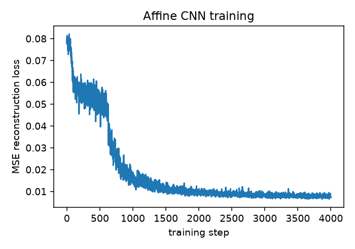
Result on the held-out benchmark: 5.26 px landmark error (both scenarios – the network never learned to fix elastic drift specifically, it just does its regular affine job on Scenario B too). Training loss dropped smoothly and plateaued around 0.007-0.008 MSE.

Training loss curve.

Registered results on both scenarios.

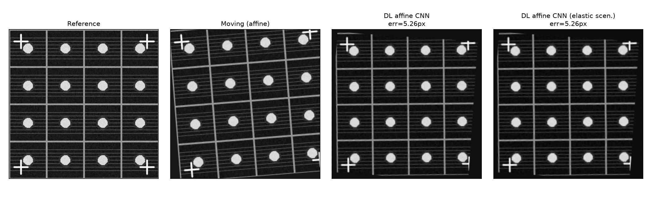
That’s an honest result, not a great one: 5.26px is roughly 100x worse than ECC’s 0.02px on the identical problem. Visually the grid is close to aligned, but a residual rotation is still visible at the corners. This makes sense once you think about what each method is actually doing: ECC re-optimizes its transform from scratch on this exact pair, refining until the correlation score stops improving. The CNN has to generalize a single set of weights across an entire distribution of possible drifts, ahead of time, without ever seeing this specific pair during training – it’s solving a harder problem (amortized inference) in exchange for a much cheaper one at test time (a single forward pass instead of an iterative per-image optimization). For a small CNN like this one, that trade shows up as reduced peak accuracy. A bigger network, more training diversity, or a coarse-to-fine architecture would likely close some of this gap – but “some of the gap,” not obviously “past ECC,” which is already sub-pixel. The honest takeaway: on a problem this well-suited to classical intensity-based optimization, training a small DL regressor doesn’t buy you accuracy – it buys you speed at scale, if you have enough recipes/volume to amortize the training cost.

0.2 Method 5: LoFTR (deep feature matching)

LoFTR (“Local Feature TRansformer”) replaces SIFT’s separate detect-then-describe pipeline with a single transformer that predicts dense correspondences directly between two images, detector-free. It’s the deep-learning generation of feature matching – same job as SIFT+RANSAC, learned instead of hand-engineered.

import kornia.feature as KF

matcher = KF.LoFTR(pretrained="outdoor").to(device).eval()

def loftr_affine(ref, moving):
    out = matcher({"image0": to_kornia(moving), "image1": to_kornia(ref)})
    mkpts0, mkpts1 = out["keypoints0"].cpu().numpy(), out["keypoints1"].cpu().numpy()
    keep = out["confidence"].cpu().numpy() > 0.5
    M, inliers = cv2.estimateAffinePartial2D(mkpts0[keep], mkpts1[keep],
                                              method=cv2.RANSAC, ransacReprojThreshold=3.0)
    return M

The honest expectation going in was a domain-gap failure: kornia’s "outdoor" LoFTR checkpoint is trained on natural photo scenes (city landmarks, outdoor structures) – nothing like this benchmark’s flat, high-contrast, synthetic line-art. That expectation was wrong, and the actual result is the most interesting one in this post.

Dense correspondences found by LoFTR between the moving and reference images.

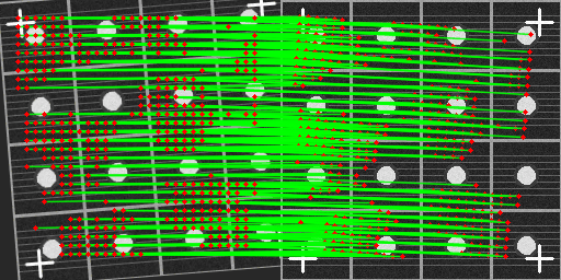
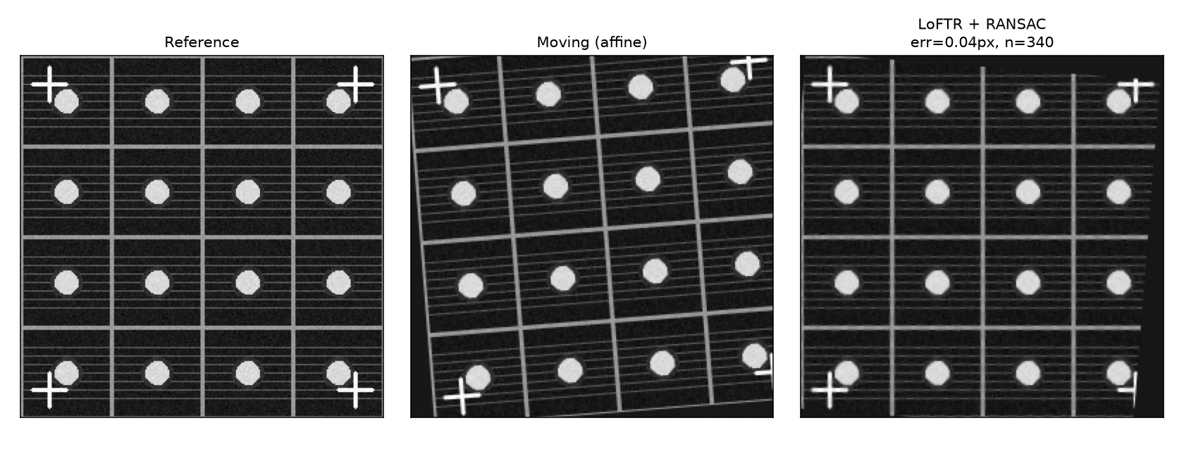
Result: 0.04 px on Scenario A, 0.19 px on Scenario B – 340 matches above 0.5 confidence (mean confidence 0.76), essentially tied with SIFT+RANSAC and ECC, and ~130x more accurate than the affine CNN this post trained from scratch specifically for this reference pattern.

Registered result.

Why did a natural-photo-pretrained matcher generalize this well to a synthetic industrial pattern? The likely reason: LoFTR’s transformer attends over broad spatial context to find geometrically consistent correspondences, and this benchmark’s crosses, circular pads, and grid intersections are unambiguous, high-contrast local structure – exactly the kind of feature LoFTR was trained to find, just rendered in a different visual style than its training photos. That’s a reasonable finding, but it is a single benchmark result, not a generalization guarantee – a real fab image with low contrast, heavy sensor noise, or genuinely textureless regions could easily land LoFTR back in its actual domain gap. The practical recommendation this result supports is “try LoFTR, validate on your real images before trusting it,” not “LoFTR always works out of the box on industrial imagery.”

0.3 Results so far

Method	Scenario A	Scenario B	Type
ECC (Part 1)	0.02 px	0.21 px	Classical, intensity-based
SIFT + RANSAC (Part 1)	0.05 px	0.20 px	Classical, feature-based
DL affine CNN	5.26 px	5.26 px	Deep learning, learned regressor
LoFTR + RANSAC	0.04 px	0.19 px	Deep learning, learned feature matching

The headline so far: the deep-learning method that replaces feature detection (LoFTR) matches classical accuracy; the one that replaces the optimizer (the affine CNN) doesn’t, at least not at this model size and training budget. Neither one, however, can touch Scenario B’s elastic component – they’re both still fundamentally fitting a single global affine matrix. Part 3 drops that constraint entirely.