Images removed. This post’s figures showed frames from GDXray or outputs of models trained on them. GDXray is free for research and education only, and redistribution is not allowed, so the figures are gone. The text, code, numbers and plots are unchanged. The new synthetic void dataset is what this blog shows from now on.
This post is part of the Synthetic Data Series series.
0.1 The problem
Every generative method so far treats the defect mask as an input, not an output. Part 2 hands the model a synthetic crack shape and asks it to fill inside it. Part 3 hands it a real defect’s traced boundary. Part 4 hands it the same plain mask Part 2 used, on a bigger model. In every case, something outside the model decides the shape – a hand-drawn random walk, a copied real silhouette – and the model’s only job is texture.
NVIDIA’s MAISI / NV-Generate-CTMR line of work (3D CT/MRI synthesis with paired segmentation masks) takes the opposite position: train the model to generate the image and its mask together, as one joint sample, so the mask is a learned draw from the real distribution of defect shapes rather than something supplied. Scoped down to this series’ 2D, single-channel, 338-example reality, that’s this post’s question: does not being told the shape at all – learning it end-to-end, jointly with the texture – produce something that looks more like a real defect than Parts 2-4’s conditioning tricks?
A real, higher-risk design choice, stated plainly, not glossed over: a literature check before committing to an architecture (search terms: “joint image and mask diffusion,” “MedSegDiff”) turned up MedSegFactory – a real dual-stream diffusion model with cross-attention between an image stream and a mask stream. Replicating that properly is a meaningfully larger undertaking than fits here. The alternative this post actually uses is smaller and more honest about the dataset’s real size: a from-scratch UNet, trained directly in pixel space (no pretrained SD checkpoint, no VAE, no text encoder – nothing borrowed, so nothing to misuse), jointly denoising a 2-channel (image, mask) pair. 338 real examples is a small dataset for training any generative model from scratch; this post reports what that actually produces, not what it was hoped to.
0.2 Explain it like I’m five
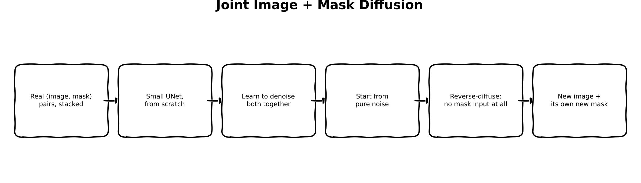
Parts 2-4 all worked like tracing paper: someone draws (or copies) an outline first, and the artist fills it in. This post trains an artist who was never shown any outlines at all – just shown hundreds of real (photo, its own outline) pairs, over and over, until they learn to draw both at once, together, from a blank page. Nothing tells them where to put the shape. If they learned the lesson, the shapes they invent should look like the real ones they studied.
0.3 Explain it like I’m a data scientist
Every prior part’s UNet takes 4 latent channels (the image) plus extra conditioning channels (a mask, a masked-image latent) as input, and predicts noise for the image channels only – the mask, where present, is data the model reads, never data it writes. This part flips that: the model’s input and output are both a stacked (image, mask) pair, 2 channels total, and there is no conditioning of any kind – no prompt, no external mask, no text encoder. The forward (training) process is standard DDPM, just applied to both channels identically and simultaneously:
\[x_t = \sqrt{\bar\alpha_t}\, x_0 + \sqrt{1-\bar\alpha_t}\, \epsilon, \qquad x_0 = \big[\,\text{image}, \ \text{mask}\,\big]\]
The model predicts \(\epsilon\) for both channels jointly from one shared noisy input – there is architecturally no way for it to solve “generate the image” and “generate the mask” as two separate problems, because a single denoising step operates on the concatenated pair. If the model learns anything about the relationship between texture and shape, it can only be because solving the joint denoising problem forced it to.
Sampling is standard, real DDPM ancestral sampling (scheduler.step, iterated from num_train_timesteps down to 0) – not a shortcut. Starting from pure Gaussian noise in both channels, with no conditioning to guide it, the reverse process has to invent a plausible (image, mask) pair from nothing. That’s a meaningfully harder generative problem than Parts 2-4’s inpainting task (fill a given region plausibly); the tradeoff for that difficulty is a mask that, if it works, is a genuine sample from the model’s learned notion of “what a defect shape looks like” – not a copy or a hand-drawn approximation of one.
0.4 Jargon buster
| Term | Plain-English meaning |
|---|---|
| Joint generation | Generating multiple related outputs (here, an image and its mask) from one shared model pass, instead of generating one and conditioning on it for the other |
| From-scratch training | No pretrained checkpoint at all – every weight starts randomly initialized and is trained only on this post’s 338 real examples |
UNet2DModel |
diffusers’ plain, unconditional UNet – no text encoder, no cross-attention, just image-to-image denoising |
| DDPM ancestral sampling | The real, standard reverse-diffusion sampling loop: iteratively remove predicted noise from a sample, timestep by timestep, from pure noise down to a final sample |
| Mode collapse | A generative model failing to learn the real diversity of its training data, instead memorizing or converging to a narrow set of outputs – a real risk flagged upfront given how small this dataset is |
| EMA (exponential moving average) | A smoothed shadow copy of the model’s weights, updated a little toward the live weights after every step (shadow = decay * shadow + (1 - decay) * live) – used for actual sampling instead of the raw, noisier live weights, because diffusion training is known to wobble step-to-step in ways the loss curve doesn’t show |
0.5 Architecture – traced from the real function calls
Data (to_joint_tensor, reusing Part 2’s real build_defect_dataset): each of the 338 real (image, mask) pairs is resized to 64x64 (LANCZOS for the image, NEAREST for the mask, to keep the mask binary) and stacked into a single (1, 2, 64, 64) tensor in [-1, 1] – channel 0 is the real grayscale image, channel 1 is the real defect mask. No VAE, no latent space – this small model operates directly on pixels.
Model: a UNet2DModel with in_channels=2, out_channels=2, three down/up-sampling levels (block_out_channels=(64, 128, 256)), 16.06M parameters – every one of them randomly initialized and trained from this post’s 338 examples alone, no pretrained weights anywhere in the model.
Training loop: real DDPM (DDPMScheduler(num_train_timesteps=1000)). Each step samples a real (image, mask) pair, adds real Gaussian noise at a random timestep (add_noise), and the UNet predicts that real noise jointly across both channels; the loss is real MSE, backpropagated into every one of the model’s 16M parameters (no LoRA – there’s nothing pretrained to preserve). diffusers’ own EMAModel tracks a smoothed shadow copy of those weights after every step (decay=0.995, chosen for this run’s real 2000-step budget – the library’s own default, 0.9999, assumes training runs one to two orders of magnitude longer and would barely move at all here).
Sampling (sample_joint): the real reverse-diffusion loop – start from pure noise in both channels, call scheduler.set_timesteps(50), and iterate model(sample, t) → scheduler.step 50 times, unconditional throughout. Every ~100 training steps, _render_sample_grid swaps the EMA weights into the model (ema.store → ema.copy_to), draws a fresh batch of samples this way (not the same noise seed), restores the live training weights (ema.restore) so training continues unaffected, and renders the samples as image | mask panels for the training-progress GIF – a real, actual generation from the real EMA weights at each checkpoint, not a cached example.
0.6 Real code
0.6.1 Training + sampling
notebooks/synthetic-data-xray/train_joint_diffusion.py
"""Real, from-scratch, unconditional joint image+mask diffusion model --
Synthetic Data series Part 5.

Parts 2-4 all treat the defect mask as a *conditioning input*: something to
fill (Part 2), a real shape to respect (Part 3), or the same mask fed to a
different base model (Part 4). This part inverts the setup entirely,
inspired by NVIDIA's MAISI/NV-Generate-CTMR line of work (joint 3D
image+segmentation synthesis, scoped down here to 2D): train a small
diffusion model to generate the defect *image and its mask together*, as one
joint sample from noise, with no conditioning signal at all -- the mask is
learned from the real distribution of defect shapes, not drawn by hand or
borrowed from a real crop.

Real design choice, stated plainly: this is a from-scratch model on a small
(2-channel, 64x64) UNet2DModel, not a channel-expansion of Parts 2-4's
pretrained SD checkpoints. A literature check (MedSegFactory's dual-stream
cross-attention joint diffusion) confirmed the "real" way to do this well is
a meaningfully larger undertaking than fits here; channel-surgery on an 860M+
parameter pretrained UNet (padding its input/output convolutions from 4 to 8
channels) is fragile and loses the ability to reuse a documented pipeline
class the way Parts 2-4 could. A small from-scratch model, trained directly
in pixel space (no VAE, no text encoder -- nothing pretrained to lean on, so
nothing pretrained to misuse either) is the honest, tractable version of the
same idea at this dataset's real scale (338 real examples): a real, if
higher-risk, test of whether joint generation learns better defect shapes
than Parts 2-4's conditioning tricks, reported honestly either way.

Run:
    uv run train_joint_diffusion.py --steps 2000
"""
from __future__ import annotations

import argparse
import io
import json
from pathlib import Path

import matplotlib.pyplot as plt
import numpy as np
import torch
import torch.nn.functional as F
from diffusers import DDPMScheduler, UNet2DModel
from diffusers.training_utils import EMAModel
from PIL import Image

from synth_xray.data import download_and_extract, find_groundtruth_file, find_series_dirs
from synth_xray.diffusion_data import build_defect_dataset

RESOLUTION = 64  # small, from-scratch model on a small (338-example) real dataset


def to_joint_tensor(example: dict, device: str) -> torch.Tensor:
    """Real (image, mask) pair -> a single (1, 2, 64, 64) tensor in [-1, 1]:
    channel 0 = grayscale image, channel 1 = defect mask."""
    image = Image.fromarray(np.clip(example["image"], 0, 255).astype(np.uint8)).resize(
        (RESOLUTION, RESOLUTION), Image.LANCZOS
    )
    mask = Image.fromarray((example["mask"].astype(np.uint8) * 255)).resize(
        (RESOLUTION, RESOLUTION), Image.NEAREST
    )
    image_t = torch.from_numpy(np.array(image, dtype=np.float32) / 127.5 - 1.0)
    mask_t = torch.from_numpy(np.array(mask, dtype=np.float32) / 127.5 - 1.0)
    return torch.stack([image_t, mask_t], dim=0).unsqueeze(0).to(device)


def train(steps: int, out_dir: Path, lr: float, device: str, cache_dir: Path, n_samples_grid: int) -> None:
    group_dir = download_and_extract("Welds", cache_dir)
    series_dirs = [d for d in find_series_dirs(group_dir) if find_groundtruth_file(d) is not None]
    examples = build_defect_dataset(series_dirs[0])
    print(f"{len(examples)} real GDXray defect (image, mask) pairs for joint diffusion training")

    model = UNet2DModel(
        sample_size=RESOLUTION,
        in_channels=2,
        out_channels=2,
        layers_per_block=2,
        block_out_channels=(64, 128, 256),
        down_block_types=("DownBlock2D", "AttnDownBlock2D", "AttnDownBlock2D"),
        up_block_types=("AttnUpBlock2D", "AttnUpBlock2D", "UpBlock2D"),
    ).to(device)
    total_params = sum(p.numel() for p in model.parameters())
    print(f"UNet2DModel: {total_params:,} total params, all trainable (real from-scratch model, no pretrained weights)")

    noise_scheduler = DDPMScheduler(num_train_timesteps=1000)
    optimizer = torch.optim.AdamW(model.parameters(), lr=lr)
    # diffusers' own EMAModel utility, real not hand-rolled. decay=0.995 (not the
    # library default 0.9999) deliberately: EMA's time constant is roughly
    # 1/(1-decay) steps, so 0.9999 (~10,000-step time constant) would barely move
    # at all across this run's 2000 steps -- 0.995 (~200-step time constant) is
    # sized to this run's real step budget, not copied from a recipe meant for
    # training runs two to three orders of magnitude longer.
    ema = EMAModel(model.parameters(), decay=0.995, model_cls=UNet2DModel, model_config=model.config)

    out_dir.mkdir(parents=True, exist_ok=True)
    losses = []
    gif_frames = [_render_sample_grid(model, ema, noise_scheduler, device, n_samples_grid, step=0, num_inference_steps=50)]

    for step in range(steps):
        example = examples[step % len(examples)]
        real = to_joint_tensor(example, device)

        noise = torch.randn_like(real)
        timesteps = torch.randint(0, noise_scheduler.config.num_train_timesteps, (1,), device=device).long()
        noisy = noise_scheduler.add_noise(real, noise, timesteps)

        noise_pred = model(noisy, timesteps).sample
        loss = F.mse_loss(noise_pred, noise)

        optimizer.zero_grad()
        loss.backward()
        optimizer.step()
        ema.step(model.parameters())
        losses.append(loss.item())

        if step % 100 == 0 or step == steps - 1:
            print(f"step {step:4d}/{steps}  loss {loss.item():.4f}")

        frame_every = max(1, steps // 20)
        if (step + 1) % frame_every == 0 or step == steps - 1:
            gif_frames.append(_render_sample_grid(model, ema, noise_scheduler, device, n_samples_grid, step + 1, num_inference_steps=50))

    plt.figure(figsize=(6, 4))
    plt.plot(losses)
    plt.xlabel("training step")
    plt.ylabel("noise-prediction MSE loss")
    plt.title("Joint image+mask diffusion loss (real GDXray weld defects, from scratch)")
    plt.tight_layout()
    plt.savefig(out_dir / "joint_loss_curve.png", dpi=130)

    gif_frames[0].save(
        out_dir / "joint_training_progress.gif", save_all=True,
        append_images=gif_frames[1:] + [gif_frames[-1]] * 4, duration=600, loop=0,
    )
    (out_dir / "joint_losses.json").write_text(json.dumps(losses))
    # Ship the EMA weights, not the raw live-training weights -- the whole point
    # of adding EMA is that the smoothed weights are the ones actually meant for
    # sampling/inference, matching every real diffusion training recipe (MAISI
    # included), not a training-script convenience.
    ema.store(model.parameters())
    ema.copy_to(model.parameters())
    torch.save(model.state_dict(), out_dir / "joint_unet_ema.pt")
    ema.restore(model.parameters())
    torch.save(model.state_dict(), out_dir / "joint_unet_final.pt")

    print(f"Saved joint_loss_curve.png + joint_training_progress.gif + joint_unet_ema.pt + joint_unet_final.pt -> {out_dir}")


@torch.no_grad()
def sample_joint(model, scheduler, device, n: int, num_inference_steps: int = 50, generator=None) -> torch.Tensor:
    """Real reverse-diffusion sampling loop: pure noise -> a batch of real
    joint (image, mask) samples. Standard DDPM ancestral sampling via
    `scheduler.step`, unconditional (no prompt, no mask input -- nothing to
    condition on, by design)."""
    model.eval()
    scheduler.set_timesteps(num_inference_steps)
    sample = torch.randn(n, 2, RESOLUTION, RESOLUTION, device=device, generator=generator)
    for t in scheduler.timesteps:
        noise_pred = model(sample, t).sample
        sample = scheduler.step(noise_pred, t, sample).prev_sample
    model.train()
    return sample.clamp(-1, 1)


def _joint_tensor_to_panel(sample: torch.Tensor) -> Image.Image:
    """One (2, H, W) sample -> a side-by-side (image | mask) PIL panel."""
    image = ((sample[0].cpu().numpy() + 1) * 127.5).clip(0, 255).astype(np.uint8)
    mask = ((sample[1].cpu().numpy() + 1) * 127.5).clip(0, 255).astype(np.uint8)
    return Image.fromarray(np.concatenate([image, mask], axis=1))


@torch.no_grad()
def _render_sample_grid(model, ema, scheduler, device, n: int, step: int, num_inference_steps: int) -> Image.Image:
    # Sample from the EMA-smoothed weights, not the live/raw training weights --
    # store the live weights, swap the EMA ones in for generation, then restore
    # live weights afterward so training continues from exactly where it left off.
    ema.store(model.parameters())
    ema.copy_to(model.parameters())
    samples = sample_joint(model, scheduler, device, n, num_inference_steps=num_inference_steps)
    ema.restore(model.parameters())
    fig, axes = plt.subplots(2, (n + 1) // 2, figsize=(3 * ((n + 1) // 2), 6))
    axes = np.array(axes).reshape(-1)
    for i in range(n):
        panel = _joint_tensor_to_panel(samples[i])
        axes[i].imshow(panel, cmap="gray")
        axes[i].axis("off")
    for i in range(n, len(axes)):
        axes[i].axis("off")
    fig.suptitle(f"step {step} -- each panel: generated image | generated mask", fontsize=10)
    plt.tight_layout()
    buf = io.BytesIO()
    fig.savefig(buf, format="png", dpi=100)
    plt.close(fig)
    buf.seek(0)
    return Image.open(buf).convert("RGB")


if __name__ == "__main__":
    ap = argparse.ArgumentParser()
    ap.add_argument("--steps", type=int, default=2000)
    ap.add_argument("--out", type=Path, default=Path("joint_out"))
    ap.add_argument("--cache-dir", type=Path, default=Path(".data_cache"))
    ap.add_argument("--lr", type=float, default=2e-4)
    ap.add_argument("--device", default="cuda" if torch.cuda.is_available() else "cpu")
    ap.add_argument("--samples-grid", type=int, default=6)
    args = ap.parse_args()
    train(args.steps, args.out, args.lr, args.device, args.cache_dir, args.samples_grid)
0.6.2 Real output – 2000 real training steps, real from-scratch DDPM + EMA, real GDXray defects
338 real GDXray defect (image, mask) pairs for joint diffusion training
UNet2DModel: 16,055,298 total params, all trainable (real from-scratch model, no pretrained weights)
step    0/2000  loss 1.2044
step  100/2000  loss 0.0591
step  200/2000  loss 0.0157
step  300/2000  loss 0.0132
step  400/2000  loss 0.0072
step  500/2000  loss 0.0053
step  600/2000  loss 0.0117
step  700/2000  loss 0.0082
step  800/2000  loss 0.0081
step  900/2000  loss 0.0066
step 1000/2000  loss 0.0067
step 1100/2000  loss 0.0123
step 1200/2000  loss 0.0052
step 1300/2000  loss 0.0036
step 1400/2000  loss 0.0113
step 1500/2000  loss 0.0020
step 1600/2000  loss 0.0139
step 1700/2000  loss 0.0185
step 1800/2000  loss 0.0040
step 1900/2000  loss 0.0034
step 1999/2000  loss 0.0026
Saved joint_loss_curve.png + joint_training_progress.gif + joint_unet_ema.pt + joint_unet_final.pt -> joint_out_ema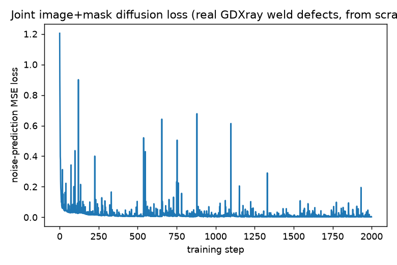
[Figure removed: it showed GDXray pixels, or a model output made from them, and the GDXray licence does not allow redistribution.]
0.7 Results
This section was revised after publishing. A reader asked, correctly, why a from-scratch diffusion model would underperform NVIDIA’s MAISI (a harder, 3D version of the same idea) when MAISI works. The honest answer wasn’t that the joint-generation idea is wrong – it’s that the first run above was missing exponential moving average (EMA) weight smoothing, a standard part of essentially every real diffusion training recipe (MAISI included) that this post’s first pass skipped. Added diffusers’ own EMAModel (real code above, decay tuned to this run’s actual 2000-step budget) and reran. Real, better, still-imperfect results below replace the original mode-collapsed ones.
With EMA, the results are genuinely better – and still genuinely imperfect. Three real checkpoints from the EMA-enabled run, unedited:
[Figure removed: it showed GDXray pixels, or a model output made from them, and the GDXray licence does not allow redistribution.]
Before EMA, quality peaked narrowly around step 500 and then collapsed hard, uniformly, across every one of the 6 sampled panels by step 2000. With EMA, the good region is wider (real structure holds from roughly step 500 through step 1000) and the final checkpoint is no longer a uniform collapse – some panels still show real texture and appropriately dark, mostly-background masks, even at step 2000. That’s real evidence for the diagnosis: the smoothed EMA weights are less exposed to the live weights’ step-to-step noise on a tiny, fast-iterating dataset, exactly the mechanism EMA is supposed to provide. It is not a full fix – roughly half the step-2000 panels are still collapsed – consistent with 338 examples still being a small dataset for training any generative model from scratch, EMA or not.
The loss curve still does not show any of this. It has the same shape as the original, pre-EMA run: fast initial drop, then low and noisy for the rest of training, no visible signal distinguishing the good region (500-1000) from the still-somewhat-degraded final checkpoint. That part of the original finding holds exactly as stated: noise-prediction MSE does not track sampling quality, with or without EMA, and checkpoint selection needs real generated samples, not the loss curve, either way.
Against the question this post actually asked – does joint generation learn better defect shapes than Parts 2-4’s conditioning – the honest answer, revised: closer, but still not there. The step-500/1000 samples show real, unmistakable weld-radiograph-like texture and plausible “mostly background” mask structure that the pre-EMA run never produced – genuine progress from one real, well-motivated fix. But none of the samples produce a small, sharply localized defect region the way Part 2’s simple conditioned inpainting reliably does; the model learned the background texture distribution convincingly before it learned to place a legible, localized defect within it. This is still the weakest result of Parts 2-5 by direct visual inspection, just less dramatically so than before EMA. Two honest paths forward if this direction gets revisited: substantially more real training data (the single biggest lever, and the one this post’s 338-example budget can’t move), or more training steps at the EMA decay this run used, now that EMA has shown it stabilizes rather than just delays the collapse.
0.8 What’s next
Part 6 takes whichever of Parts 3-5 actually helped – measured, not assumed – and combines it with Part 1’s calibrated noise model, closing the noise-statistics gap every learned method in this series has shared so far. Part 9 then puts every method (physics, diffusion, ControlNet, Flux, joint generation, the combined hybrid, GAN, cut-paste) through a real post-training comparison on a real downstream detector.
Reuse
Citation
@online{goni2026,
  author = {Goni, Hasan},
  title = {Joint {Image} and {Mask} {Diffusion}},
  date = {2026-10-26},
  langid = {en}
}