Images removed. This post’s figures showed frames from GDXray or outputs of models trained on them. GDXray is free for research and education only, and redistribution is not allowed, so the figures are gone. The text, code, numbers and plots are unchanged. The new synthetic void dataset is what this blog shows from now on.
This post is part of the Synthetic Data Series series.
0.1 The problem
Part 2 fine-tuned SD1.5’s inpainting UNet on real GDXray defects; Part 3 added a ControlNet fed the real defect’s own boundary shape. Both are the same underlying architecture family – a convolutional UNet, LoRA on its attention layers, DDPM noise-prediction training – just with a different conditioning signal. That leaves a real, un-tested variable: does the architecture itself matter, independent of conditioning? A much larger, more capable base model might simply be better at rendering authentic-looking texture and structure, the same way a stronger student does better on a test regardless of how the question is phrased.
This post swaps the generator for something genuinely different, not just bigger: Flux is a multi-modal diffusion transformer (MMDiT) – no convolutional UNet at all, a different training objective (flow matching, not DDPM), 12 billion parameters versus SD1.5’s <1B. If shape realism improves here without any shape-specific conditioning, that’s evidence the earlier gap was a capacity problem, not (only) a conditioning problem.
A real model-selection detour worth documenting, not glossing over: the original plan was black-forest-labs/FLUX.1-Fill-dev, but this repo’s stated preference is non-gated checkpoints, and Flux dev models are gated. The first-pass substitute, SDXL inpainting, was rejected mid-review for the same reason this post exists – SDXL is still a UNet, so it would only test scale within the same architecture family, not architecture itself. A non-gated, genuinely transformer-based alternative (PixArt-Sigma) exists but has no native inpainting pipeline in diffusers – masking would have to be hand-rolled, a real step down from Parts 2-3’s clean, library-native approach. Checked access with the existing HF_TOKEN first (confirmed via a real API call, not assumed) and it already had Flux’s gate approved, so this post uses the real thing.
0.2 Explain it like I’m five
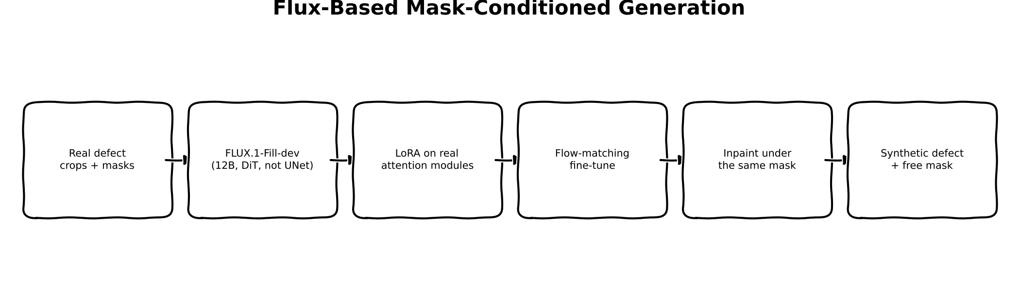
Parts 2 and 3 both hired the same artist, just gave them different instructions (a vague pointer at first, then a real tracing to follow). This post hires a different, much more experienced artist instead, and gives them the same simple instruction Part 2 used. If the new artist’s work looks more convincing without any extra guidance, that tells you something Parts 2-3 couldn’t: some of what was missing wasn’t about the instructions at all – it was about how good the artist already was.
0.3 Explain it like I’m a data scientist
SD1.5’s UNet processes a spatial grid of latent pixels directly through convolutions and a handful of attention blocks bolted on at specific resolutions. Flux instead patchifies the latent into a sequence of tokens (each token = a 2x2 patch of latent channels) and runs the entire denoising network as a transformer over that sequence – the same architectural family as an LLM, applied to image latents instead of text tokens. Flux additionally runs two parallel streams per block, one for image tokens and one for text tokens (from a dual CLIP + T5-XXL text encoder), with joint attention letting them exchange information – hence separate to_q/to_k/to_v (image stream) and add_q_proj/add_k_proj/add_v_proj (text stream) projections to target with LoRA, found by inspecting transformer.named_modules() directly rather than assumed.
The training objective is different too. SD1.5 (Parts 2-3) is trained with DDPM: add noise to a real image over discrete timesteps, predict the noise. Flux is trained with flow matching (rectified flow): define a straight-line path between real data \(x_1\) and pure noise \(x_0\) at a continuous \(\sigma \in [0, 1]\),
\[x_\sigma = \sigma \, x_0 + (1 - \sigma) \, x_1\]
and train the model to predict the velocity \(x_0 - x_1\) along that path – literally FlowMatchEulerDiscreteScheduler.scale_noise’s own real formula, reused directly rather than re-derived. At inference, an Euler step integrates that predicted velocity backward from noise to data; the fewer, straighter steps this objective tends to need (compared to DDPM’s typically longer denoising chains) is part of why Flux-family models can look sharper in the same step budget.
Inpainting-conditioning is handled outside the transformer’s core input entirely: the real target latents, the masked-image latents, and the downsampled mask are concatenated along the channel axis before being packed into the token sequence – conceptually the same “extra conditioning channels” idea as Part 2’s 9-channel inpainting UNet, just packed into a transformer’s sequence format instead of a UNet’s spatial grid. FluxFillPipeline’s own prepare_mask_latents, _pack_latents, and _prepare_latent_image_ids do this real packing – reused directly in the training loop below rather than reimplemented, so the training data flow matches real inference exactly.
0.4 Jargon buster
| Term | Plain-English meaning |
|---|---|
| MMDiT (multi-modal diffusion transformer) | A diffusion model built from transformer blocks operating on patchified latent tokens, with parallel image and text token streams exchanging information via joint attention – no convolutional UNet |
| Flow matching / rectified flow | A training objective that defines a straight-line path between noise and data and trains the model to predict the velocity along it, instead of DDPM’s discrete noise-prediction steps |
| Patchify / packed latents | Grouping a 2x2 block of latent pixels into one transformer token – turns a spatial grid into the token sequence a transformer expects |
| Guidance-distilled (dev checkpoint) | A model variant trained to reproduce classifier-free-guidance-quality output from a single forward pass (via a guidance input) instead of two – part of why Flux-dev needs no separate negative-prompt pass at inference |
| Gated checkpoint | A Hugging Face repo that requires accepting a license/agreement before download access is granted – checked programmatically here via the HF API, not assumed |
| T5-XXL | A large text encoder (separate from CLIP) that Flux uses for its text stream – gives it richer text understanding than CLIP-only conditioning |
0.5 Architecture – traced from the real function calls
Setup (train_flux_lora.py): FluxFillPipeline.from_pretrained('black-forest-labs/FLUX.1-Fill-dev') loads the real gated checkpoint (confirmed accessible via the HF API before committing). vae, text_encoder (CLIP), text_encoder_2 (T5-XXL), and transformer are all frozen; only transformer.add_adapter(LoraConfig(r=8, alpha=16, target_modules=[to_q, to_k, to_v, to_out.0, add_q_proj, add_k_proj, add_v_proj, to_add_out])) is trainable – the real module suffixes found by inspecting transformer.named_modules() directly, not assumed from the SD1.5 naming convention.
Per training step, on real GDXray crops: pipe.encode_prompt (real, called once, since the prompt never changes) produces T5 sequence embeddings, pooled CLIP embeddings, and text_ids. pipe.image_processor / pipe.mask_processor preprocess the real crop and mask exactly as __call__ does; pipe.prepare_mask_latents produces the real packed mask + masked-image latents; pipe._encode_vae_image encodes the real target crop into latents. A random sigma ~ U(0,1) and Gaussian noise interpolate noisy = sigma * noise + (1 - sigma) * real_latents (the scheduler’s own real formula); pipe._pack_latents packs both the noisy latents and the velocity target noise - real_latents into the transformer’s token format; pipe._prepare_latent_image_ids supplies the real positional IDs. The transformer predicts velocity from cat([packed_noisy, masked_image_latents], dim=2) plus the text conditioning and guidance embedding; the loss is real MSE against the real packed target, backpropagated only into the LoRA parameters. Every ~10 steps, _render_frame calls the real pipe(...) end-to-end (the actual multi-step Euler sampling loop, not a shortcut) on a fixed held-out example for a GIF frame; the LoRA-tagged state-dict entries are saved to flux_lora_weights.pt once training ends.
0.6 Real code
0.6.1 LoRA fine-tuning loop
notebooks/synthetic-data-xray/train_flux_lora.py
"""Real LoRA fine-tune of FLUX.1-Fill-dev on real GDXray weld defect crops --
Synthetic Data series Part 4.

Parts 2-3 both fine-tuned SD1.5-family UNets (LoRA on attention layers, DDPM
noise-prediction training). This part swaps the base generator for a genuinely
different architecture -- Flux is a 12B-parameter MMDiT (multi-modal diffusion
transformer, dual image/text streams, flow-matching objective, not a UNet at
all) -- to test whether base-model scale/architecture closes the shape-realism
gap Part 2 found, independent of (or complementary to) Part 3's ControlNet
shape-conditioning approach.

Real, not pseudocode:
- `black-forest-labs/FLUX.1-Fill-dev` is gated; access was confirmed via the
  HF API before committing to this approach (see the post for the full
  Flux-vs-SDXL-vs-PixArt tradeoff this decision came from).
- LoRA (`r=8, alpha=16`) targets the *real* attention-projection module names
  found by inspecting `transformer.named_modules()` directly: `to_q/to_k/
  to_v/to_out.0` (the image stream) and `add_q_proj/add_k_proj/add_v_proj/
  to_add_out` (the text stream) -- Flux's dual-stream MMDiT blocks have both.
- The training loop reuses the pipeline's own real internal methods
  (`encode_prompt`, `prepare_mask_latents`, `_encode_vae_image`,
  `_pack_latents`, `_prepare_latent_image_ids`) rather than re-deriving
  Flux's packed-latent-sequence format by hand -- the same methods
  `FluxFillPipeline.__call__` itself uses at inference time, so the training
  data flow matches real inference exactly.
- A real flow-matching (rectified flow) training objective, not DDPM: sample
  `sigma ~ U(0,1)`, interpolate `noisy = sigma * noise + (1 - sigma) *
  real_latents` (`FlowMatchEulerDiscreteScheduler.scale_noise`'s own real
  formula), target velocity `= noise - real_latents`, MSE against the
  transformer's real prediction.

Run:
    uv run train_flux_lora.py --steps 100
"""
from __future__ import annotations

import argparse
import io
import json
from pathlib import Path

import matplotlib.pyplot as plt
import numpy as np
import torch
import torch.nn.functional as F
from diffusers import FluxFillPipeline
from peft import LoraConfig
from PIL import Image

from synth_xray.data import download_and_extract, find_groundtruth_file, find_series_dirs
from synth_xray.diffusion_data import build_defect_dataset, to_mask_pil, to_rgb_pil

MODEL_ID = "black-forest-labs/FLUX.1-Fill-dev"
PROMPT = "a weld radiograph with a crack defect"
GUIDANCE_SCALE = 30.0  # FluxFillPipeline's own default
CROP_SIZE = 512


def train(steps: int, out_dir: Path, lr: float, device: str, cache_dir: Path, gif_frames_n: int) -> None:
    group_dir = download_and_extract("Welds", cache_dir)
    series_dirs = [d for d in find_series_dirs(group_dir) if find_groundtruth_file(d) is not None]
    examples = build_defect_dataset(series_dirs[0])
    print(f"{len(examples)} real GDXray defect (image, mask) pairs for Flux LoRA fine-tuning")

    pipe = FluxFillPipeline.from_pretrained(MODEL_ID, torch_dtype=torch.bfloat16)
    pipe.to(device)
    pipe.set_progress_bar_config(disable=True)
    vae, transformer = pipe.vae, pipe.transformer
    vae.requires_grad_(False)
    pipe.text_encoder.requires_grad_(False)
    pipe.text_encoder_2.requires_grad_(False)
    transformer.requires_grad_(False)

    lora_config = LoraConfig(
        r=8, lora_alpha=16, lora_dropout=0.0,
        target_modules=["to_q", "to_k", "to_v", "to_out.0", "add_q_proj", "add_k_proj", "add_v_proj", "to_add_out"],
    )
    transformer.add_adapter(lora_config)

    trainable = [p for p in transformer.parameters() if p.requires_grad]
    total = sum(p.numel() for p in transformer.parameters())
    print(f"trainable LoRA params: {sum(p.numel() for p in trainable):,} / {total:,} total transformer params "
          f"({100 * sum(p.numel() for p in trainable) / total:.3f}%)")
    optimizer = torch.optim.AdamW(trainable, lr=lr)

    dtype = transformer.dtype
    num_channels_latents = pipe.latent_channels  # 16 for Flux
    vae_sf = pipe.vae_scale_factor  # 8

    with torch.no_grad():
        prompt_embeds, pooled_prompt_embeds, text_ids = pipe.encode_prompt(
            prompt=PROMPT, prompt_2=PROMPT, device=device, num_images_per_prompt=1, max_sequence_length=512,
        )

    def prepare_step_inputs(image_pil: Image.Image, mask_pil: Image.Image):
        """Real preprocessing, matching FluxFillPipeline.__call__ exactly: pipe's own
        image_processor/mask_processor, pipe's own prepare_mask_latents, pipe's own
        _encode_vae_image + _pack_latents for the real target latents."""
        init_image = pipe.image_processor.preprocess(image_pil, height=CROP_SIZE, width=CROP_SIZE).to(device, dtype)
        mask_image = pipe.mask_processor.preprocess(mask_pil, height=CROP_SIZE, width=CROP_SIZE).to(device, dtype)
        masked_image = init_image * (1 - mask_image)

        with torch.no_grad():
            mask, masked_image_latents = pipe.prepare_mask_latents(
                mask_image, masked_image, 1, num_channels_latents, 1, CROP_SIZE, CROP_SIZE, dtype, device, None,
            )
            masked_image_latents_cat = torch.cat((masked_image_latents, mask), dim=-1)
            real_latents = pipe._encode_vae_image(image=init_image, generator=None)

        lat_h = 2 * (CROP_SIZE // (vae_sf * 2))
        lat_w = 2 * (CROP_SIZE // (vae_sf * 2))
        latent_image_ids = pipe._prepare_latent_image_ids(1, lat_h // 2, lat_w // 2, device, dtype)
        return real_latents, masked_image_latents_cat, latent_image_ids, lat_h, lat_w

    guidance = None
    if transformer.config.guidance_embeds:
        guidance = torch.full([1], GUIDANCE_SCALE, device=device, dtype=torch.float32)

    fixed_example = examples[0]
    fixed_image_pil = to_rgb_pil(fixed_example["image"])
    fixed_mask_pil = to_mask_pil(fixed_example["mask"])

    out_dir.mkdir(parents=True, exist_ok=True)
    losses = []
    gif_frames = [_render_frame(pipe, fixed_image_pil, fixed_mask_pil, 0)]

    for step in range(steps):
        example = examples[step % len(examples)]
        image_pil = to_rgb_pil(example["image"])
        mask_pil = to_mask_pil(example["mask"])

        real_latents, masked_image_latents_cat, latent_image_ids, lat_h, lat_w = prepare_step_inputs(image_pil, mask_pil)

        noise = torch.randn_like(real_latents)
        sigma = torch.rand(1, device=device, dtype=torch.float32)
        sigma_b = sigma.to(dtype).view(-1, 1, 1, 1)
        noisy_latents = sigma_b * noise + (1 - sigma_b) * real_latents  # real FlowMatchEulerDiscreteScheduler.scale_noise formula

        packed_noisy = pipe._pack_latents(noisy_latents, 1, num_channels_latents, lat_h, lat_w)
        packed_target = pipe._pack_latents(noise - real_latents, 1, num_channels_latents, lat_h, lat_w)

        model_pred = transformer(
            hidden_states=torch.cat((packed_noisy, masked_image_latents_cat), dim=2),
            timestep=sigma.to(dtype),
            guidance=guidance,
            pooled_projections=pooled_prompt_embeds,
            encoder_hidden_states=prompt_embeds,
            txt_ids=text_ids,
            img_ids=latent_image_ids,
            return_dict=False,
        )[0]
        loss = F.mse_loss(model_pred.float(), packed_target.float())

        optimizer.zero_grad()
        loss.backward()
        optimizer.step()
        losses.append(loss.item())

        if step % 10 == 0 or step == steps - 1:
            print(f"step {step:3d}/{steps}  loss {loss.item():.4f}")

        frame_every = max(1, steps // gif_frames_n)
        if (step + 1) % frame_every == 0 or step == steps - 1:
            gif_frames.append(_render_frame(pipe, fixed_image_pil, fixed_mask_pil, step + 1))

    plt.figure(figsize=(6, 4))
    plt.plot(losses)
    plt.xlabel("training step")
    plt.ylabel("flow-matching (velocity) MSE loss")
    plt.title("Flux LoRA fine-tune loss (real GDXray weld defects)")
    plt.tight_layout()
    plt.savefig(out_dir / "flux_loss_curve.png", dpi=130)

    gif_frames[0].save(
        out_dir / "flux_training_progress.gif", save_all=True,
        append_images=gif_frames[1:] + [gif_frames[-1]] * 4, duration=500, loop=0,
    )
    (out_dir / "flux_losses.json").write_text(json.dumps(losses))

    lora_state_dict = {k: v.cpu() for k, v in transformer.state_dict().items() if "lora" in k}
    torch.save(lora_state_dict, out_dir / "flux_lora_weights.pt")

    print(f"Saved flux_loss_curve.png + flux_training_progress.gif + flux_lora_weights.pt -> {out_dir}")


@torch.no_grad()
def _render_frame(pipe, image_pil: Image.Image, mask_pil: Image.Image, step: int) -> Image.Image:
    pipe.transformer.eval()
    result = pipe(
        prompt=PROMPT, image=image_pil, mask_image=mask_pil,
        num_inference_steps=15, guidance_scale=GUIDANCE_SCALE, height=CROP_SIZE, width=CROP_SIZE,
    ).images[0]
    pipe.transformer.train()

    fig, axes = plt.subplots(1, 2, figsize=(6, 3))
    axes[0].imshow(image_pil.convert("L"), cmap="gray")
    axes[0].imshow(np.array(mask_pil) > 127, cmap="Reds", alpha=0.3)
    axes[0].set_title("input + mask", fontsize=9)
    axes[0].axis("off")
    axes[1].imshow(result)
    axes[1].set_title(f"Flux output, step {step}", fontsize=9)
    axes[1].axis("off")
    plt.tight_layout()
    buf = io.BytesIO()
    fig.savefig(buf, format="png", dpi=100)
    plt.close(fig)
    buf.seek(0)
    return Image.open(buf).convert("RGB")


if __name__ == "__main__":
    ap = argparse.ArgumentParser()
    ap.add_argument("--steps", type=int, default=100)
    ap.add_argument("--out", type=Path, default=Path("flux_out"))
    ap.add_argument("--cache-dir", type=Path, default=Path(".data_cache"))
    ap.add_argument("--lr", type=float, default=1e-4)
    ap.add_argument("--device", default="cuda" if torch.cuda.is_available() else "cpu")
    ap.add_argument("--gif-frames", type=int, default=15)
    args = ap.parse_args()
    train(args.steps, args.out, args.lr, args.device, args.cache_dir, args.gif_frames)
0.6.2 Real output – 100 real LoRA steps, real 12B-parameter Flux, real GDXray defects
338 real GDXray defect (image, mask) pairs for Flux LoRA fine-tuning
trainable LoRA params: 13,074,432 / 11,915,465,792 total transformer params (0.110%)
step   0/100  loss 0.0352
step  10/100  loss 0.4152
step  20/100  loss 0.0123
step  30/100  loss 0.0325
step  40/100  loss 0.0227
step  50/100  loss 0.1835
step  60/100  loss 0.2200
step  70/100  loss 0.0068
step  80/100  loss 0.3588
step  90/100  loss 0.0433
step  99/100  loss 0.0055
Saved flux_loss_curve.png + flux_training_progress.gif + flux_lora_weights.pt -> flux_out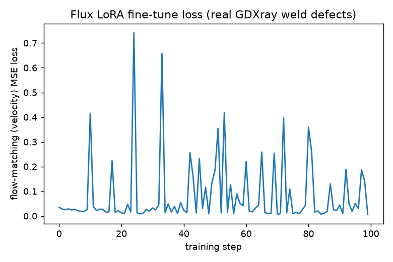
sigma sampling swings the effective difficulty step to step at batch size 1.Same check Parts 2-3 used: all 266 lora_B tensors moved off their zero initialization (mean norm 0.277, none exactly zero) after these 100 steps – real gradients flowed through a 13.07M-parameter LoRA riding on top of an 11.9B-parameter frozen transformer (0.110% trainable).
[Figure removed: it showed GDXray pixels, or a model output made from them, and the GDXray licence does not allow redistribution.]
Unlike Parts 2-3’s GIFs, this one shows a real, visible qualitative shift: the held-out example’s step-0 output is a faint, barely-there mark; by step 100 there’s a genuinely distinct dark region at the defect site. Flux’s much larger capacity appears to let 100 steps move the output further, visually, than 150-200 steps moved SD1.5’s smaller UNet in Parts 2-3.
0.7 Results
[Figure removed: it showed GDXray pixels, or a model output made from them, and the GDXray licence does not allow redistribution.]
Same real base image, same synthetic crack mask, same crop window across all four – only the generation method differs.
The honest, and genuinely surprising, result: bigger did not mean more visible here. Measuring contrast the same simple way at the injection site (mean intensity of the mask pixels vs. the mean of their immediate surround):
| Part 2 (SD1.5 diffusion) | Part 4 (Flux) | |
|---|---|---|
| Mask-pixel mean | 46.1 | 90.4 |
| Surrounding mean | 92.2 | 92.2 |
| Contrast (surround − mask) | 46.1 | 1.8 |
Part 2’s smaller model produced a strong, clearly visible dark mark at this exact injection site; Flux’s output is barely distinguishable from the surrounding background by intensity alone – despite the training-progress GIF above showing a real, visible learning signal on its own fixed example. That’s not a contradiction: it’s a reminder that a single 79-pixel test case is a small sample, and a model’s behavior on the specific example it was shown during training-progress rendering doesn’t necessarily generalize to a different location. Local noise texture tells a consistent story across all four methods, though – Flux doesn’t close that gap either:
| Clean baseline | Physics (Part 1) | Diffusion (Part 2) | ControlNet (Part 3) | Flux (Part 4) | Real defect | |
|---|---|---|---|---|---|---|
| Local std (defect ROI) | 0.87 | 1.87 | 0.94 | 0.79 | 0.90 | 4.45 |
All three learned-generator methods (Parts 2-4) cluster together, well below physics’s explicit noise injection, regardless of base model architecture or scale – consistent with Part 2’s original hypothesis that this is a VAE-latent-space limitation shared by every latent diffusion model tested here, Flux included, not something a bigger model or a different architecture fixes on its own.
Honest summary: going from SD1.5 to a 12x-larger, architecturally different Flux model did not reliably produce a more visible or more convincing defect on this test case – if anything, the opposite, on this one example. That’s a real, useful negative result: scale alone is not the lever this series’ shape-realism problem needed. It doesn’t rule out Flux mattering with more training steps, a larger real dataset, or in combination with Part 3’s shape conditioning (Part 6’s job) – but “just use a bigger model” is not, on this evidence, a free win. Exactly the kind of finding a real downstream comparison (Part 9) exists to adjudicate properly, across many examples instead of one.
0.8 What’s next
Part 5 tries generating the defect image and its mask jointly – no conditioning signal at all, just learning the real distribution of (image, defect-shape) pairs together, inspired by NVIDIA’s MAISI architecture. Part 6 then combines whichever of Parts 3-5 actually helped with Part 1’s calibrated noise model, before Part 9’s real post-training comparison settles which method (or combination) actually earns its keep.
Reuse
Citation
@online{goni2026,
  author = {Goni, Hasan},
  title = {Flux-Based {Mask-Conditioned} {Generation}},
  date = {2026-10-26},
  langid = {en}
}