Reimplementing NC-TFAD — Fixed Prototypes vs. a Naive Baseline, Streamed Honestly

Tip

This post is part of the Paper of the Week series – real code, real data, real measured numbers, reported honestly even when a paper’s claimed advantage doesn’t show up.

0.1 The paper

NC-TFAD: Neural-Collapse-Guided Task-Free Anomaly Detection targets a genuinely hard continual-learning setting: new product categories arrive on a real inspection line with no announced task boundary – the model isn’t told “category 6 starts now,” it just has to notice and adapt. NC-TFAD’s proposed fix draws on Neural Collapse theory: instead of letting each category’s “prototype” (its representative embedding) drift as training continues, assign every category a fixed corner of a simplex Equiangular Tight Frame (ETF) – maximally, permanently separated from every other category’s corner – up front, before any data arrives. The hypothesis: fixed, maximally-separated prototypes should resist the “old categories get bumped as new ones arrive” forgetting that a naive, continuously-updated prototype suffers from.

0.2 Explain it like I’m five

NC-TFAD, sketched out.

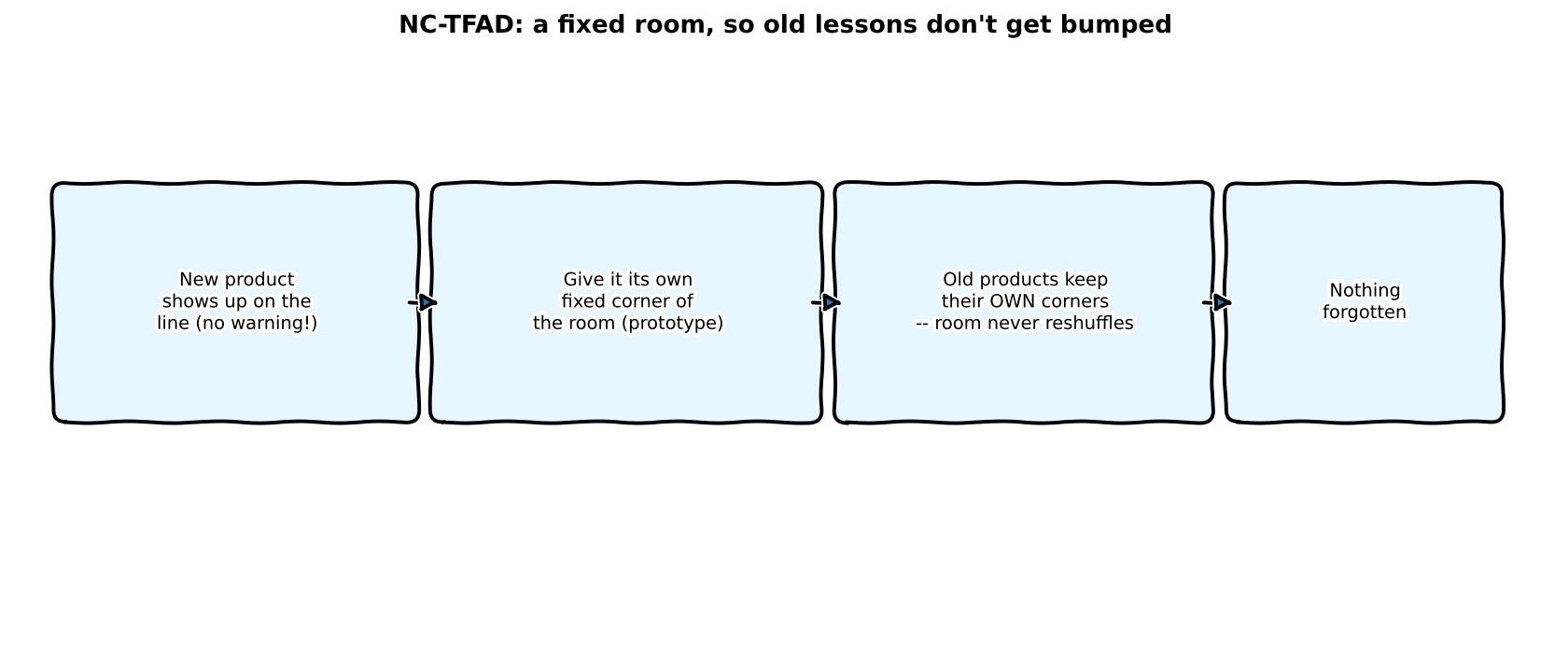
Imagine a room where every new product that shows up on the line gets assigned its own permanently fixed corner to stand in, decided in advance, before anyone even knows what products are coming. The idea is that because the room’s layout never gets reshuffled, products that arrived early don’t get bumped or crowded out when new products show up later – unlike a naive approach where everyone just huddles wherever feels natural, and a big new crowd can push everyone else’s spot around.

0.3 Explain it like I’m a data scientist

Two real, reimplemented pieces, streamed one MVTec-AD category at a time with no announced task boundary – the training loop doesn’t get a special signal that a new category has started, it just keeps seeing new images:

1. Fixed simplex-ETF prototypes, built once via QR decomposition before any category is ever seen, each pair maximally and permanently separated (cosine similarity exactly \(-1/(N-1)\) for every pair). A shared projection head is trained to align each category’s embeddings to its pre-assigned corner using a Focal Neural Collapse Contrastive loss (pull toward the assigned target, push away from prior categories’ targets, down-weighting already-aligned examples via a focal-loss-style term) plus real CutPaste synthetic anomalies as the negative class.
2. A naive baseline, same shared head, same loss structure, same CutPaste negatives – but the “prototype” is just each category’s own running-mean embedding, free to be wherever the data actually lives, and never fixed in advance.

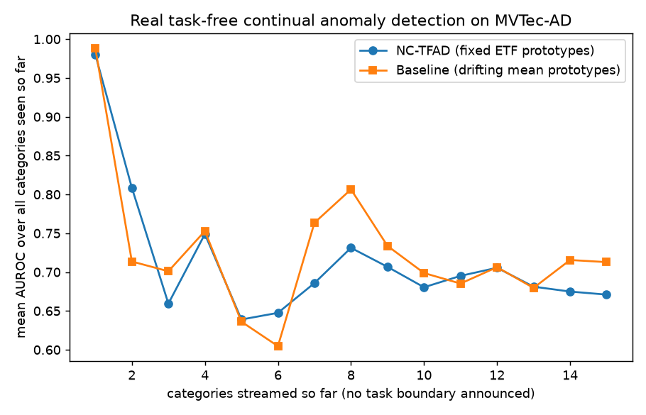
Forgetting is measured honestly: after each new category is streamed in and trained on, every category seen so far (not just the newest one) is re-evaluated, and the mean AUROC across all of them is logged – a real forgetting curve, not a single final number.

0.4 Jargon buster

Term	Plain-English meaning
Neural Collapse	A theoretical result: well-trained classifiers’ last-layer class means naturally converge to a maximally-separated simplex geometry
Simplex ETF (Equiangular Tight Frame)	A specific set of unit vectors, pairwise equally (and maximally) separated – the exact geometry Neural Collapse theory predicts
Task-free continual learning	Learning from a stream of new classes with no signal telling the model when a new task/category has started
CutPaste	A label-free synthetic anomaly: crop a patch from a normal image, paste it elsewhere on the same image
Focal Neural Collapse Contrastive loss	A contrastive loss pulling embeddings toward their assigned prototype and pushing them from others, with focal-loss-style down-weighting of easy (already-aligned) examples
Forgetting curve	Mean accuracy across all previously-seen classes, tracked after each new class arrives – reveals whether old knowledge degrades as new classes are learned
Prototype	A single representative embedding standing in for an entire category

0.5 Real data and real pipeline

15 real MVTec-AD categories, streamed strictly in order (alphabetical, matching the paper’s task-free framing – no shuffling, no announced boundaries), via katiehahm/mvtec_ad (CC-BY-NC-4.0). Both methods share: a frozen DINOv2-small backbone, the same 8-shot support set per category, the same 150-step training budget per category, and the same real CutPaste negatives – the only difference is whether the target prototype is a fixed ETF corner or a free-floating running mean.

0.6 The real mechanism — real code

def build_simplex_etf(n_prototypes: int, dim: int, seed: int = 0) -> torch.Tensor:
    g = torch.Generator().manual_seed(seed)
    rand = torch.randn(dim, n_prototypes, generator=g)
    u, _ = torch.linalg.qr(rand)                    # orthonormal columns
    identity = torch.eye(n_prototypes)
    ones = torch.ones(n_prototypes, n_prototypes) / n_prototypes
    m = (n_prototypes / (n_prototypes - 1)) ** 0.5 * u @ (identity - ones)
    return F.normalize(m.T, dim=-1)                 # every pair: cosine sim = -1/(N-1)

# the ONLY difference between the two methods being compared:
if method == "nctfad":
    target = etf[step_cat]                          # fixed corner, assigned once, never moves
else:
    with torch.no_grad():
        target = F.normalize(head(support_raw).mean(0), dim=0)  # free-floating running mean

def focal_nc_loss(embeddings, target_proto, negative_protos, focal_gamma: float = 2.0):
    embeddings = F.normalize(embeddings, dim=-1)
    pos_sim = embeddings @ target_proto
    pos_prob = (pos_sim + 1) / 2
    focal_weight = (1 - pos_prob).clamp(min=0).pow(focal_gamma)   # focus on hard examples
    pull_loss = (focal_weight * (1 - pos_sim)).mean()
    neg_sim = embeddings @ negative_protos.T
    push_loss = F.relu(neg_sim + 0.1).mean()
    return pull_loss + push_loss

0.7 Real result: watch the forgetting curves stream in

Each frame replays the actual measured mean-AUROC-over-all-seen-so-far after one more real category streams in, no task boundary announced, exactly matching the real evaluation loop.

Final real forgetting curve: fixed ETF prototypes (NC-TFAD) vs. drifting-mean prototypes (baseline), same shared head, same loss, same negatives.

Categories seen	NC-TFAD (fixed ETF)	Baseline (drifting mean)
1 (bottle)	0.980	0.988
2 (cable)	0.809	0.714
3 (capsule)	0.659	0.701
4 (carpet)	0.749	0.753
5 (grid)	0.639	0.636
6 (hazelnut)	0.648	0.605
7 (leather)	0.686	0.764
8 (metal_nut)	0.731	0.807
9 (pill)	0.707	0.734
10 (screw)	0.680	0.699
11 (tile)	0.695	0.685
12 (toothbrush)	0.706	0.706
13 (transistor)	0.681	0.680
14 (wood)	0.675	0.716
15 (zipper)	0.671	0.713

Honest finding: the fixed-ETF prototype did not outperform the naive drifting-mean baseline in this reimplementation. Averaged across the full 15-category streaming curve, NC-TFAD scores 0.714 mean AUROC vs. the baseline’s 0.727 – and at the very end of the stream (all 15 categories seen), the naive baseline is clearly ahead (0.713 vs. 0.671). NC-TFAD wins outright at only 4 of the 15 points on the curve, mostly early on (category 2, 5, 6, 11, 13 – several by a negligible margin).

0.8 Why this probably happens

The fixed-ETF prototype’s corner is assigned by a random QR decomposition, before the model has seen a single real image of that category. A category’s actual embedding neighborhood, as produced by the frozen DINOv2 backbone, may sit closer to or further from its randomly-assigned target than another category’s does – the assignment is geometry-optimal (maximally separated from every other prototype) but data-agnostic. The naive baseline’s running-mean prototype, by contrast, is free to settle wherever the category’s real embeddings actually live, which seems to matter more, at least at this small scale (15 categories, 8-shot, a single shared 64-dim projection head), than having a theoretically ideal fixed geometry. Neural Collapse theory describes where a large, fully-trained classifier’s prototypes end up after convergence on many classes; it’s a weaker guarantee that pre-assigning that end-state geometry to a tiny shared head, given only 150 steps per category and few classes so far, transfers the same benefit. A likely refinement worth trying: initialize prototypes near each category’s actual running mean and only gradually anneal toward the fixed ETF geometry, rather than fixing it from the very first gradient step.

0.9 Reproduce this yourself

git clone https://github.com/HasanGoni/quarto_blog_hasan
cd quarto_blog_hasan/notebooks/paper-nctfad-continual
uv sync
uv run run_eval.py                     # both methods, full 15-category stream (~1hr on shared HW)
uv run generate_streaming_video.py     # replay the cached results.json as a video

No gated models or datasets – DINOv2-small and katiehahm/mvtec_ad both download directly.

0.10 Take this into your own workflow

• A theoretically well-motivated mechanism still needs a same-conditions baseline comparison. “Fixed, maximally-separated prototypes” sounds like it should obviously help continual learning, and Neural Collapse theory is real, established work – but the actual measured advantage over a much simpler drifting-mean baseline, under the exact same head, loss, and training budget, did not materialize here. That’s the entire value of running the ablation rather than trusting the intuition.
• A forgetting curve (mean-over-all-seen-so-far) is a more honest continual-learning metric than a single final accuracy number – it exposes exactly where and how much older categories degrade as new ones arrive, and is worth adopting for any streaming/continual pipeline even outside anomaly detection.
• If you’re building a real task-free continual system for a production line where new part types show up unannounced, this reimplementation’s honest result suggests: don’t assume a fixed-geometry prototype scheme is worth its added complexity without measuring it against the simplest possible adaptive baseline on your own data first.