Reimplementing PL-SCEA — Take Two, After a GitHub Issue Told Me I Got It Wrong

Tip

This post is part of the Paper of the Week series – real code, real data, real measured numbers, reported honestly even when they don’t flatter the paper.

WarningCorrection (2026-10-04)

The first version of this post was wrong, and I’ve rewritten it from scratch. A GitHub issue opened by ysinjoro-coder pointed out two mistakes – the paper’s default is γ = 2 (not 4), and its backbone is RADIOv3 (not DINO). Checking the paper’s full text against my code, it was worse than that: I had also dropped the per-token standardization and applied the reweighting to the block’s output instead of inside its attention. The old headline – “PL-SCEA dropped mean AUROC from 0.831 to 0.739” – described a method that isn’t PL-SCEA, and I retract it. Thank you for the report.

0.1 What was wrong the first time

	The paper (arXiv:2609.03655)	My first version (wrong)	This version
Backbone	frozen RADIOv3-B	DINOv2-small	frozen C-RADIOv3-B (nvidia/C-RADIOv3-B)
Power exponent γ	2 by default (ablated in Fig. 5)	4.0, “per the paper”	2 (and 4, and a sweep)
Correlation	cosine similarity, then per-token standardization (Eq. 5-6), keep only above-average	raw cosine, relu, self masked	standardized, max(0, ·)^γ (Eq. 7)
Where it’s applied	replaces attention in the final block: weights from Y = softmax(QK^T/√d)·V, re-aggregate the original V (Eq. 1-10)	after the fact, on the block’s output tokens	hooked inside the final block’s attention, exactly Eq. 1-10
Fallback	a token with no positive relation keeps itself (Eq. 8)	none	identity fallback
Anomaly head	VAE, cosine loss, 64-d latent, AdamW 8e-4, noise, standardized scores	tiny MSE VAE, 32-d	the paper’s recipe (details below)

0.2 The paper

PL-SCEA: Reconfiguring Pretrained Attention for Few-Shot Industrial Anomaly Detection argues that a frozen vision foundation model’s last attention layer is tuned for semantic aggregation (“what object is this?”), not for exposing small local defects. PL-SCEA keeps the pretrained query-key attention only to build semantically conditioned values, then derives a new attention map from how those values correlate with each other, token by token – with no new trainable attention parameters. A small VAE (“Latent Normality Modeling”) is then fit on the reconfigured patch features of a handful of normal images, and reconstruction error is the anomaly score.

0.3 Explain it like I’m five

PL-SCEA, sketched out.

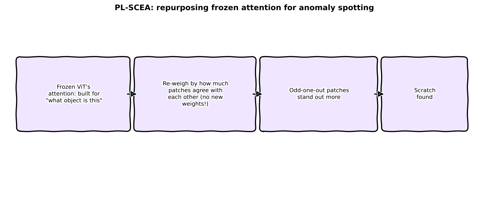
Picture a classroom where every student asks “who in this room thinks like I do?” – but each student only listens to the classmates they agree with more than they agree with the average person, and listens extra hard to their very closest friends. A class that’s mostly in consensus ends up looking even more uniform. A genuine mistake (an anomaly) has no real friends to average toward, so it keeps sticking out.

0.4 Explain it like I’m a data scientist

Let \(X\) be the patch tokens entering the final attention layer. Per head, the original attention gives contextualized values \(Y = A_{qk}V\). PL-SCEA uses \(Y\) only to measure relations:

\[ \tilde y_i = \frac{y_i}{\lVert y_i\rVert},\quad S = \tilde Y\tilde Y^\top,\quad \hat S_{ij} = \frac{S_{ij}-\mu_i}{\sigma_i+\epsilon},\quad R_{ij} = \max(0,\hat S_{ij})^{\gamma},\quad A^{\text{PL-SCEA}}_{ij} = \frac{R_{ij}}{\sum_j R_{ij}} \]

and then re-aggregates the original values, \(O = A^{\text{PL-SCEA}}V\). The key idea is the standardization: \(\mu_i,\sigma_i\) are the mean and std of token \(i\)’s own row of \(S\), so “positive” means “more related to me than the typical token is” – a token-adaptive threshold. The exponent \(\gamma\) then decides how winner-takes-all the surviving relations are.

A concrete example: say a token’s similarities to five peers are \([0.9, 0.8, 0.5, 0.4, 0.3]\). The row mean is \(0.58\), std \(\approx 0.23\), so the standardized scores are \([+1.4, +0.9, -0.3, -0.8, -1.2]\). Only the first two survive the \(\max(0,\cdot)\). With \(\gamma = 2\) their weights come out at roughly \(68\%/32\%\); with \(\gamma = 4\) at roughly \(82\%/18\%\). Bigger \(\gamma\) = a more “winner takes all” average. (My first version never did this standardization: with raw cosines, almost every peer survives, which is a very different operation.)

0.5 Jargon buster

Term	Plain-English meaning
Frozen backbone	A pretrained feature extractor used as-is, no fine-tuning. Here: C-RADIOv3-B, a model distilled from several teachers (CLIP-, DINOv2-, SAM-style) into one
Contextualized value (\(Y = A_{qk}V\))	Each token’s value vector after mixing in its neighbors using the ordinary attention weights – “what this token means in context”
Token-adaptive standardization	Judging each token’s correlations against its own average, not one global threshold
Power-law reweighting	Raising the surviving scores to the power \(\gamma\) so the strongest relations dominate the weighted average
Latent Normality Modeling (LNM)	A small VAE fit on a few normal images; anomalies reconstruct badly
Few-shot anomaly detection	Deciding “defective or fine?” after seeing only a handful (1-8) of normal examples
AUROC / AUPR	How well anomaly scores rank real defective images above real normal ones (AUPR: with “defective” as the positive class)
QK attention (baseline)	The model’s own, unmodified last-layer attention – the control in every comparison below

0.6 Architecture: where PL-SCEA sits

The code below follows the data through the real library calls, no pseudocode:

• AutoModel.from_pretrained("nvidia/C-RADIOv3-B", trust_remote_code=True) loads the frozen encoder. Its trunk is a 12-block timm ViT (model.model.blocks), patch size 16, with a handful of prefix tokens (CLS + registers) in front of the patch tokens.
• The last block’s attn is a stock timm.models.vision_transformer.Attention (qkv → softmax(QK) → proj). I replace only its forward with a version that has two modes: "qk" (the original computation, verified identical to the stock module to ~3e-7) and "plscea".
• In "plscea" mode the prefix tokens still get the ordinary attention output; the patch tokens get A_PL-SCEA @ V built from the standardized, power-law-reweighted self-correlation of Y = softmax(QK^T/√d) V, computed per head.
• The block’s residual, LayerNorm, MLP and all earlier blocks are untouched. The 28×28 = 784 patch tokens that come out (448×448 input) are L2-normalized and fed to the VAE head.
• The VAE (LNM): L2-normalized feature + Gaussian noise → re-normalize → encoder → 64-d latent → decoder; loss = cosine reconstruction + β·KL. At test time it is deterministic: encode the clean feature, decode the posterior mean, anomaly score = 1 − cosine(feature, reconstruction), standardized by the training patches’ score statistics.

Because the same frozen weights are used for both modes, every comparison below changes exactly one thing: the final block’s attention.

0.7 The real mechanism – real code

def plscea_weights(y: torch.Tensor, gamma: float) -> torch.Tensor:
    """Paper Eq. 3-9. y: (B, H, N, d) contextualized values of the PATCH tokens only."""
    y_n = F.normalize(y, dim=-1, eps=EPS)                      # Eq. 3: L2-normalize tokens
    s = y_n @ y_n.transpose(-2, -1)                            # Eq. 4: cosine self-correlation
    mu = s.mean(dim=-1, keepdim=True)                          # Eq. 5: per-token mean / std
    sigma = s.std(dim=-1, keepdim=True, unbiased=False)
    s_hat = (s - mu) / (sigma + EPS)                           # Eq. 6: token-adaptive standardization
    r = F.relu(s_hat).pow(gamma)                               # Eq. 7: above-average only, power-law
    d = r.sum(dim=-1, keepdim=True)                            # Eq. 8: row-normalize ...
    eye = torch.eye(r.shape[-1], device=r.device, dtype=r.dtype)
    return torch.where(d > 0, r / d.clamp_min(1e-12), eye)     # ... identity fallback

def _attn_forward(self, x, attn_mask=None, is_causal=False):    # replaces timm Attention.forward
    B, N, C = x.shape
    qkv = self.qkv(x).reshape(B, N, 3, self.num_heads, self.head_dim).permute(2, 0, 3, 1, 4)
    q, k, v = qkv.unbind(0)
    attn = ((q * self.scale) @ k.transpose(-2, -1)).softmax(dim=-1)
    y = attn @ v                                               # Eq. 1-2: Y = A_qk V
    if self.scea_mode == "plscea":
        p = N - GRID * GRID                                    # prefix (cls/register) tokens
        a_pl = plscea_weights(y[:, :, p:], self.scea_gamma)
        y = torch.cat([y[:, :, :p], a_pl @ v[:, :, p:]], dim=2)  # Eq. 10: O = A_PL-SCEA V
    out = y.transpose(1, 2).reshape(B, N, self.attn_dim)
    return self.proj_drop(self.proj(self.norm(out)))

radio = Radio(device)                               # frozen C-RADIOv3-B, final-block attention hooked
support_qk = torch.cat([radio.patch_tokens(img, "qk")     for img in shots])   # k normal images
support_pl = torch.cat([radio.patch_tokens(img, "plscea", gamma=2.0) for img in shots])

lnm_qk, mean_qk, std_qk = fit_lnm(support_qk)       # same head, same shots, run twice
lnm_pl, mean_pl, std_pl = fit_lnm(support_pl)

score = image_score(patch_score_map(lnm_pl, mean_pl, std_pl, radio.patch_tokens(test_img, "plscea")))

0.8 Two data protocols (and why there are two)

My first attempt used a Hugging Face mirror (katiehahm/mvtec_ad) that only ships MVTec-AD’s test split. So I ran everything twice:

• Setup A – test-split holdout. k “good” test images per category are held out as the few-shot support set; the rest of the test images are evaluated. Score map smoothed with σ = 1 on the 28×28 patch grid. This is what I had; it is not the paper’s protocol.
• Setup B – official protocol (closer to the paper). Support set drawn from the official train/good images; evaluation on the full official test set (good + defective, 1,725 images over 15 categories); score map upsampled to 448 px and Gaussian-smoothed with σ = 4 as in AnomalyDINO, whose preprocessing the paper follows. Data from the foersben/mvtec-ad mirror (original MVTec layout, CC BY-NC-SA 4.0).

Both: 3 support-set seeds (0, 1, 2), same seeds and same shots for every variant, the paper’s VAE recipe (cosine loss, 64-d latent, AdamW lr 8e-4, wd 1e-5, batch 512, 600 epochs), image score = mean of the top 1% of patch scores, metrics = image-level AUROC and AUPR macro-averaged over the 15 categories, reported as mean ± std over the seeds.

0.8.1 What is still different from the paper

I’d rather list these than let the numbers imply a faithful reproduction:

• VAE details the paper doesn’t give – hidden width (512), input-noise std (0.05) and β (1e-3) are my choices, and I train a fixed 600 epochs rather than “up to 600”.
• AnomalyDINO’s PCA background masking and rotation augmentation aren’t implemented.
• Smoothing / top-1% ordering is my reading of the description (upsample → σ = 4 → mean of the top 1% of pixels), not the authors’ code.
• Different support images than the paper’s seeds, naturally.
• Pixel-level metrics are only measured in setup B (official protocol), not in setup A – the paper’s largest claimed gains are pixel-level, so I added that evaluation after the first publication of this rewrite (see “Pixel level” below).
• My baseline is weaker than theirs. My QK-attention control gets 91.5 image AUROC at 1-shot and 95.9 at 8-shot (setup B), vs. the paper’s 96.5 (QK, 1-shot ablation) and 98.0 (PL-SCEA, 8-shot); at pixel level my 1-shot QK control gets 94.5 / 51.6 / 88.4 (AUROC / F1-max / PRO) vs. the paper’s 97.1 / 61.5 / 93.6. So my head/pipeline does not reach the paper’s absolute level, and everything below is conditional on this pipeline.

0.9 Results

0.9.1 8-shot, setup B (official protocol)

Per-category image AUROC, original QK attention vs. PL-SCEA (γ = 2), 8-shot, official MVTec-AD protocol, 3 seeds.

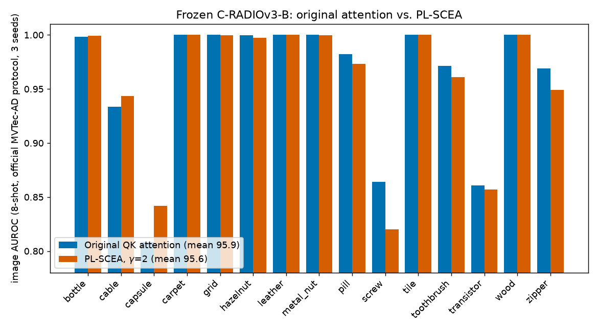
Category	QK (original)	PL-SCEA γ=2	PL-SCEA γ=4	Δ (γ=2 − QK)
bottle	99.8	99.9	99.9	+0.1
cable	93.3	94.3	93.8	+1.0
capsule	80.8	84.2	82.8	+3.4
carpet	100.0	100.0	100.0	+0.0
grid	100.0	100.0	100.0	-0.0
hazelnut	100.0	99.7	99.9	-0.2
leather	100.0	100.0	100.0	+0.0
metal_nut	100.0	100.0	100.0	-0.0
pill	98.2	97.3	97.1	-0.9
screw	86.4	82.0	83.9	-4.4
tile	100.0	100.0	100.0	+0.0
toothbrush	97.1	96.1	96.5	-1.0
transistor	86.1	85.7	84.1	-0.4
wood	100.0	100.0	100.0	+0.0
zipper	96.9	94.9	95.4	-2.0
macro AUROC, mean ± std over seeds	95.91 ± 0.75	95.62 ± 0.81	95.57 ± 0.65	-0.29
macro AUPR	97.31	97.16	97.16	-0.15

Six categories are saturated at ~100 for every variant. Among the rest, PL-SCEA helps capsule (+3.4) and cable (+1.0) and hurts screw (-4.4) and zipper (-2.0). The macro difference (-0.29) is smaller than the seed-to-seed std (~0.8), so on this pipeline PL-SCEA is a wash at 8-shot, not a clear win and not the collapse my first version reported. γ = 2 is slightly better than γ = 4 on average, which is the direction the paper’s ablation predicts.

0.9.2 8-shot, setup A (test-split holdout) – same story

	QK (original)	PL-SCEA γ=2	PL-SCEA γ=4
macro AUROC, mean ± std over seeds	97.05 ± 0.34	96.90 ± 0.27	96.76 ± 0.30

Per category it is the same pattern: capsule +2.3 and cable +0.4 up; screw -2.4, pill -1.1 down (full per-category numbers are in notebooks/paper-plscea-anomaly/out/setupA_test_holdout/). Absolute scores are higher than in setup B (the holdout is an easier protocol – the support images come from the same pool as the test images), but the PL-SCEA-vs-QK difference is again within noise.

0.9.3 The γ sweep – what the issue’s plot showed, and what I get

The issue included the paper’s Fig. 5: image-level AUROC and AUPR as the power exponent \(\gamma\) varies, both peaking at \(\gamma = 2\). Here is the same experiment on my pipeline (1-shot, 15 categories, 3 seeds; dotted lines = the original QK attention):

γ sweep, setup B (official protocol), 1-shot. AUROC (blue) and AUPR (orange) vs. the power exponent; dotted lines are the original QK attention.

γ sweep, setup A (test-split holdout), 1-shot.

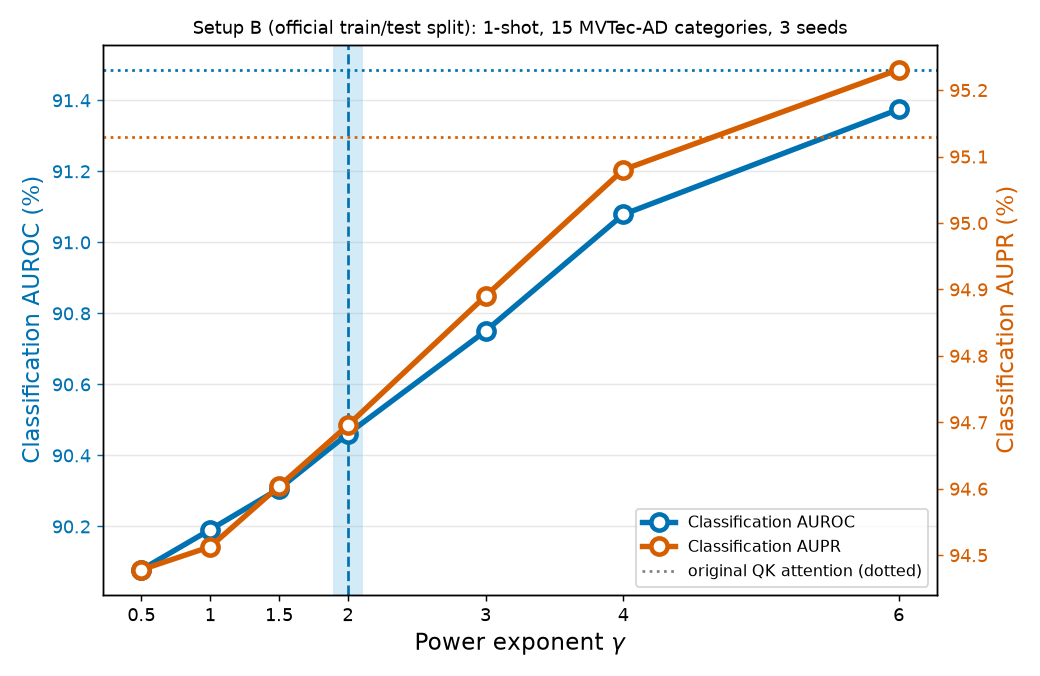
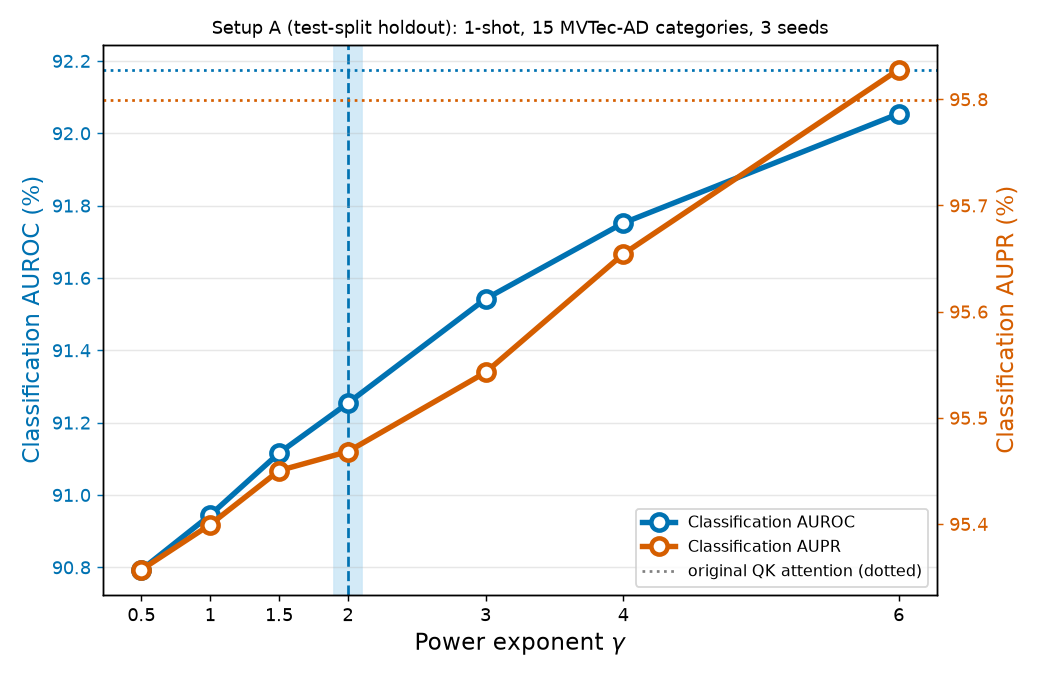
This does not reproduce the paper’s peak at γ = 2. In both setups AUROC and AUPR rise steadily with γ and are still climbing at γ = 6. In setup B (AUROC): 90.08 (γ=0.5) → 90.46 (γ=2) → 91.08 (γ=4) → 91.37 (γ=6), against 91.49 for the original attention; AUPR crosses the QK line at γ = 6 (95.23 vs 95.13). Everything is within ~1.4 points and the seed std is ~0.2-0.3 here, so it is a small, consistent trend rather than noise – but it is a trend toward the baseline, with PL-SCEA never clearly beating it.

0.9.4 Pixel level – where the paper says the gains are

The paper’s biggest claimed gains are at the pixel level (its Table 3, 1-shot, single seed: pixel F1-max 61.54 → 65.32, +3.78; pixel AUROC +0.44; PRO +0.19). So I also scored my anomaly maps against the official MVTec-AD ground-truth masks: pixel AUROC, pixel F1-max, and PRO (per-region overlap, integrated up to a false-positive rate of 0.3), per category over all test images, macro-averaged over the 15 categories, setup B, same shots and seeds as above (1-shot and 8-shot):

Shots	Metric	QK (original)	PL-SCEA γ=2	Δ (mean of per-seed differences)
1-shot	pixel AUROC	94.46 ± 0.13	94.18 ± 0.16	-0.27
1-shot	pixel F1-max	51.58 ± 0.44	54.06 ± 0.33	+2.48
1-shot	PRO	88.43 ± 0.33	87.10 ± 0.21	-1.33
8-shot	pixel AUROC	96.87 ± 0.17	97.08 ± 0.23	+0.22
8-shot	pixel F1-max	56.12 ± 0.81	58.28 ± 0.74	+2.16
8-shot	PRO	91.84 ± 0.32	91.60 ± 0.23	-0.24

Per-category change in pixel F1-max, PL-SCEA (γ = 2) minus the original attention, official protocol, mean of 3 seeds.

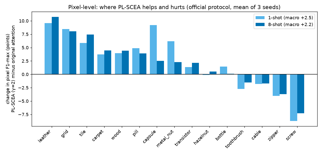
Here the paper’s direction does show up – for one metric.

• Pixel F1-max improves, consistently. +2.5 at 1-shot and +2.2 at 8-shot, positive in every one of the 3 seeds (per-seed differences +2.2 to +2.6 at 1-shot, +2.1 to +2.3 at 8-shot), with 10-11 of 15 categories improved. That is the same sign as the paper’s +3.78, a bit smaller in size.
• Pixel AUROC and PRO do not reproduce the paper’s small gains. Pixel AUROC is -0.3 at 1-shot and +0.2 at 8-shot; PRO is lower with PL-SCEA (-1.3 and -0.2). The paper reports +0.44 and +0.19 at 1-shot.
• Who wins and who loses is not random. The gains are largest on the textures – leather (+9.6 / +10.7 F1-max at 1-/8-shot), grid, tile, carpet, wood – and the losses are on objects with small, distinct structures: screw (-8.7 / -7.3), zipper, cable, toothbrush. My (untested) reading: pulling each patch toward the patches most like it sharpens the boundary of a defect on a repetitive texture, but washes out a small part-level detail on an object where nearly every patch is unique.
• Why F1-max can move while AUROC doesn’t: F1-max rewards a sharply-localized, high-contrast region at the best single threshold, whereas pixel AUROC and PRO weigh the whole ranking (all the low-scoring background and every region equally), so a reconfiguration can sharpen the top of the map without improving the overall ordering.

So, at the pixel level, a real but modest F1-max gain that depends strongly on the object category – not the across-the-board improvement the paper’s headline tables suggest, and it still comes from a baseline that is several points weaker than the paper’s.

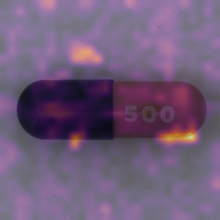
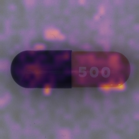
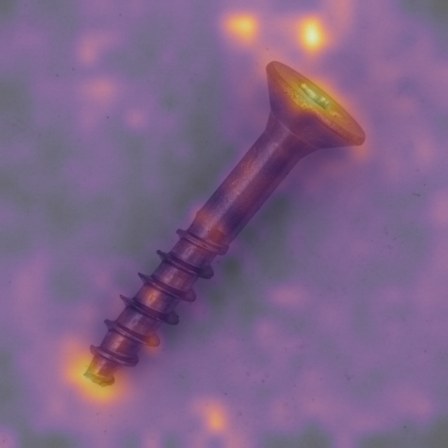
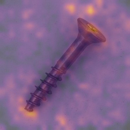
0.9.5 What the maps look like

Seed-0 anomaly maps from the same VAE heads (8-shot, setup B), original attention vs. PL-SCEA (γ = 2), on real defective images. First capsule, the category where PL-SCEA helps most:

left: PL-SCEA (γ = 2)  |  right: original QK attention -- drag to compare (same real defective capsule, shared color scale)

And screw, where it hurts most:

left: PL-SCEA (γ = 2)  |  right: original QK attention -- drag to compare (same real defective screw, shared color scale)

0.10 So what can I actually conclude?

• It depends on the metric. On this reimplementation, PL-SCEA is within noise of the original last-layer attention for image-level detection (8-shot: 95.9 vs 95.6 AUROC), and gives a consistent, modest gain in pixel F1-max (+2.2 to +2.5 points, same sign in every seed) while pixel AUROC and PRO are flat to slightly worse. Not “PL-SCEA is bad”, and not “PL-SCEA works as advertised everywhere”.
• The gain is category-dependent. Texture categories (leather, grid, tile, carpet, wood) gain the most; objects with small, distinct structures (screw, zipper, cable, toothbrush) lose. A macro average hides that split.
• I could not reproduce the γ = 2 optimum. Image-level AUROC and AUPR rise with γ up to 6 and never clearly pass the baseline. I don’t know whether that is my VAE hyperparameters (unspecified in the paper), the missing masking/augmentation, my smoothing/scoring choices, or a genuine difference. I did not rerun the γ sweep at pixel level, where the paper’s gains live, so γ = 2 may behave differently on F1-max than it does on the image metrics I swept.
• My pipeline is below the paper’s absolute numbers (2-5 image-AUROC points; ~3-10 points at pixel level), so a gap I fail to see could be hiding in whatever my head does worse. Anyone wanting to adjudicate this should run the authors’ code on the official split rather than rely on this post.
• The correction mattered a lot. The same idea went from “-9 AUROC points” (wrong implementation) to “-0.3, within noise” at image level and “+2 F1-max” at pixel level (right mechanism). A reimplementation that silently differs from the paper in the details that define the method can generate a confident, wrong verdict.

0.11 Reproduce this yourself

git clone https://github.com/HasanGoni/quarto_blog_hasan
cd quarto_blog_hasan/notebooks/paper-plscea-anomaly
uv sync
# official MVTec-AD layout (train/good + test/*), ~5 GB, to ./data/mvtec_ad:
uv run python -c "from huggingface_hub import snapshot_download as s; s('foersben/mvtec-ad', repo_type='dataset', local_dir='data/mvtec_ad', allow_patterns=['*/train/good/*','*/test/*/*'])"
uv run run_eval.py official 8 2,4                      # setup B, 8-shot, gamma 2 and 4
uv run run_eval.py official 1 0.5,1,1.5,2,3,4,6        # setup B, 1-shot gamma sweep
uv run run_eval.py holdout 8 2,4                       # setup A (needs katiehahm/mvtec_ad)
# pixel level needs the official ground-truth masks too (~1,258 small PNGs):
uv run python -c "from huggingface_hub import snapshot_download as s; s('foersben/mvtec-ad', repo_type='dataset', local_dir='data/mvtec_ad', allow_patterns=['*/ground_truth/*/*'])"
uv run run_pixel.py 1 8                                # pixel AUROC / F1-max / PRO, 1- and 8-shot
uv run generate_plots.py && uv run generate_heatmap_viz.py capsule && uv run generate_heatmap_viz.py screw

nvidia/C-RADIOv3-B and both dataset mirrors download without gating (trust_remote_code=True is required for RADIO’s model code). Runs checkpoint per category and resume if killed. Raw results (per-category, per-seed image AUROC/AUPR and pixel AUROC/F1-max/PRO) are in out/.

0.12 Take this into your own workflow

• Reimplement the formula, not the vibe. Standardization, the fallback branch, and where in the network the operation sits are part of the method. Dropping them produced a plausible-looking but wrong experiment – and a confident blog post about it.
• When a reimplementation disagrees with a paper, say which parts you matched and which you didn’t. The list under “What is still different” is more useful to a reader than a clean headline either way.
• Check the author’s ablation before trusting your own default. The paper’s γ ablation was a one-figure check that would have caught my γ = 4.
• Evaluate at the granularity the paper claims its gain at. Image-level numbers alone made PL-SCEA look like a wash; its modest F1-max gain only showed up once I scored the maps against the pixel masks. A method can be flat on one metric and useful on another.
• Run your control through the identical pipeline. The QK-attention baseline here shares weights, head, shots and seeds with PL-SCEA, which is what makes the “within noise” statement meaningful.