Reimplementing Marigold V2 — One Forward Pass, and the Fine-Tuned Checkpoint That Made Things Worse

Note

Images removed. This post’s figures showed frames from GDXray or outputs of models trained on them. GDXray is free for research and education only, and redistribution is not allowed, so the figures are gone. The text, code, numbers and plots are unchanged. The new synthetic void dataset is what this blog shows from now on.

Tip

This post is part of the Paper of the Week series – same standard as every deep-dive here: real code, real data, a real measured result, no pseudocode.

0.1 The paper

Marigold V2: Revisiting Diffusion Transformers for Monocular Depth Estimation – Igor Pavlovic, Thiemo Wandel, Anton Obukhov, Luca Bartolomei, Andrey Davydov, Fabio Tosi, Matteo Poggi, Sabine Süsstrunk, Dengxin Dai (EPFL / Huawei Bayer Lab / University of Bologna, ACM Transactions on Graphics, SIGGRAPH Asia 2026).

Marigold V1 turned a Stable-Diffusion image generator into a monocular depth estimator by fine-tuning it to denoise a depth map instead of an RGB image – clever, but still needed dozens of denoising steps to get a clean result. Marigold V2’s move: repurpose a much larger, already-excellent image editing diffusion transformer (Qwen-Image-Edit-2509) instead of a generator, LoRA-fine-tune it cheaply (rank-128 adapters, under a week on one consumer GPU), and collapse inference to a single forward pass at a fixed timestep – no iterative denoising at all. The same recipe produces depth, surface normals, albedo, and even “see-through” layered depth, and hits state-of-the-art zero-shot accuracy on the usual benchmarks (NYUv2, KITTI, ETH3D, ScanNet, DIODE).

This post reimplements the actual mechanism end to end with the real released checkpoints, and then points it at something the paper never touches: real semiconductor X-rays from lfm2-vl-xray-defects, this blog’s own GDXray+ Castings defect-detection repo from earlier in this series.

0.2 Explaining in easy word

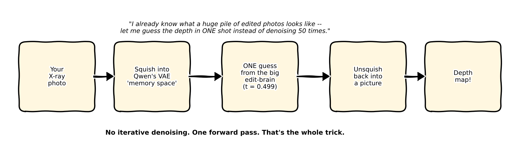
Imagine an artist who has spent years learning to edit photos – turn day into night, add a hat, remove a person. That artist has such a good mental model of what real photos look like that if you ask them “just guess how far away everything in this photo is, right now, no sketching it out first,” they can do it in one confident stroke. That’s Marigold V2: it takes an editing artist and asks it one new kind of question, and because the artist already understands photos so well, one guess is enough.

No iterative denoising – one forward pass through the transformer at a fixed timestep is the whole trick.

0.3 Jargon explanation in easy word

Term	Plain-English meaning (with real-life example to clarify)
Diffusion Transformer (DiT)	A transformer-based diffusion model backbone (uses transformers instead of the older U-Net approach). Imagine you’re building towers with Lego: U-Net is like building them layer by layer, always the same way, while Transformer is like a friend who jumps around and intelligently chooses which brick to put next. Qwen-Image-Edit-2509 uses this new Transformer-based approach.
LoRA (Low-Rank Adaptation)	Keeps the huge original model “frozen” and only trains a small, flexible add-on, which is lightweight and easy to switch around. Think of it like buying shoe inserts: instead of remaking the whole shoe for each need, you just slip in a different insert for comfort or performance. In Marigold V2, LoRA adapters let you cheaply and quickly switch tasks.
Rectified flow / flow-matching	A training method that learns the direct “straight-line path” from noisy input to clean answer, skipping lots of steps. It’s like finding a shortcut to your destination instead of taking a winding, step-by-step path. That’s why Marigold V2 can get its answer in just one step at the right “moment.”
Affine-invariant depth	The predicted depth map gets “the shape of the scene” correct, but the overall scale and brightness might be shifted. It’s like copying a drawing so all the objects are in the correct spots, but the whole image might be zoomed-in or dimmer—unless you calibrate it separately. Relative distances are right, just not the actual units.
Precomputed prompt embeddings	Instead of having to “rethink” the question every time by running a big text analyzer, Marigold V2 saves a fixed “translation” of the question (“predict the depth of this image”) and reuses it every time. Like copying your shopping list for every trip, so you don’t have to rewrite it from scratch. This skips loading the huge text encoder and speeds things up.
iREPA	A special trick used during training (not needed when using the model) that encourages Marigold V2 to notice fine details by comparing its “thoughts” to those of a very smart external image analyzer. Picture a student checking their notes against a teacher’s summary before handing in an assignment. This keeps the final result sharp.
SinkLoss	Another training-only loss, used to help the model’s VAE decoder make sharper, more realistic outputs by comparing the distribution of its results to what’s best for the “transport” (like comparing how efficiently you can move packages from one spot to another). Think of this like optimizing delivery routes at the last stage to make sure each package (pixel) arrives in the sharpest, most accurate spot.

No U-Net, no scheduler loop, no CFG – tracing the actual calls in the real huawei-bayerlab/marigold-v2 inference code:

• The base model is untouched: Qwen/Qwen-Image-Edit-2509’s own VAE (AutoencoderKLQwenImage) and transformer (QwenImageTransformer2DModel) are loaded straight from the Hub with local_files_only=True – no fine-tuned base weights, only LoRA deltas layered on top via peft.
• The RGB input is encoded exactly like an edit source image: the X-ray, normalized to [-1, 1], goes through the frozen Qwen VAE encoder and is renormalized by the VAE’s own per-channel latent mean/std – the identical preprocessing Qwen-Image-Edit uses for the image it’s about to edit.
• The text encoder is never loaded. Depth, normals, and albedo each have one fixed instruction baked into a precomputed (prompt_embeds, prompt_mask) pair, downloaded as .pt files. At inference this is loaded once and reused for every image – the live Qwen2.5-VL text encoder (~17 GB by itself) is entirely absent from the runtime graph.
• One transformer call at a fixed timestep. The encoded latent is packed into the transformer’s patch format and run through QwenImageTransformer2DModel.forward() exactly once, at a hardcoded timestep t = 0.499 – not scheduled, not sampled, the literal constant used during training. The velocity-parameterized output is converted directly to a predicted clean latent in one arithmetic step, which is the entire reason no denoising loop is needed.
• Decode and colorize. The predicted latent goes back through the same VAE’s decoder (in the paper’s default depth/Log-stage2 checkpoint, this decoder itself is LoRA/fully fine-tuned for sharper edges) to produce a raw depth-encoded RGB image, which a spectral colormap step then turns into the familiar blue-to-red depth visualization.

The upshot: Marigold V2’s “architecture” is really an inference-graph deletion exercise on top of an existing, excellent image editor – delete the text encoder, delete the denoising loop, keep the VAE and the transformer, swap in LoRA weights per task.

0.4 Real data: this blog’s own open-source X-ray dataset

Three real, held-out crops from the GDXray+ Castings subset used throughout the local-ai-defect-inspection series and lfm2-vl-xray-defects – 768×572 grayscale aluminum automotive-casting X-rays, none of them seen during Marigold V2’s training (which never touches X-ray data at all):

• C0008_0011.png – a real casting with a real annotated defect box [456, 502, 489, 545] (a small void/porosity region)
• C0008_0012.png – same series, adjacent frame, real defect box [459, 483, 489, 524]
• C0002_0001.png – a real defect-free casting from a different series, for contrast

ImportantData fit – what this post is and isn’t claiming

This is not a recommendation to deploy Marigold LoRA on X-rays, and we did not fine-tune anything on GDXray. Marigold V2 was trained on synthetic RGB indoor/outdoor scenes (Hypersim, vKITTI) with dense per-pixel depth, normal, and albedo maps. GDXray Castings gives grayscale X-rays + defect bounding boxes – the right labels for detection VLMs in Part 3, not for Marigold.

What we actually did: run the released Marigold V2 LoRA checkpoints zero-shot on held-out X-ray crops, then ask whether the adapter helps or hurts vs the frozen base model. Case 2 shows all three released modalities (depth, normals, albedo) through the fine-tuned checkpoint; Case 3 compares depth and normals only against the no-adapter baseline – that’s where the counter-intuitive result lives.

0.5 Real code

Everything below is the real script from notebooks/paper-marigold-v2/ – collapsed by default; click the summary line to expand.

Show download_assets_min.py

download_assets_min.py

# Only what inference actually touches: the base VAE + transformer (skip the
# ~17 GB text encoder), plus depth / normals / albedo LoRA checkpoints.
import os
from pathlib import Path

os.environ.setdefault("HF_HUB_DOWNLOAD_TIMEOUT", "60")
os.environ.setdefault("HF_HUB_ETAG_TIMEOUT", "30")

from huggingface_hub import snapshot_download

REPO_ROOT = Path(__file__).resolve().parent / "repo"
CKPT_DIR = REPO_ROOT / "assets" / "checkpoints"

print("[1/2] Qwen-Image-Edit-2509 base (transformer + vae only)", flush=True)
snapshot_download(
    repo_id="Qwen/Qwen-Image-Edit-2509",
    repo_type="model",
    local_dir=str(CKPT_DIR / "Qwen-Image-Edit-2509"),
    allow_patterns=[
        "model_index.json",
        "scheduler/*",
        "transformer/*",
        "vae/*",
    ],
    max_workers=1,
)

print("[2/2] Marigold-V2 LoRA checkpoints (depth + normals + albedo)", flush=True)
snapshot_download(
    repo_id="huawei-bayerlab/marigold-v2-0",
    repo_type="model",
    local_dir=str(CKPT_DIR / "Marigold-V2"),
    allow_patterns=[
        "depth/Log-stage2/*",
        "normals/*",
        "albedo/*",
        "qwen_text_embeddings/*",
        "manifest.json",
    ],
    max_workers=1,
)

print("[done]", flush=True)

Show run_inference.sh

run_inference.sh

# The real, unmodified authors' CLI -- depth, normals, and albedo on our X-rays.
set -euo pipefail
cd "$(dirname "${BASH_SOURCE[0]}")"

uv run python repo/scripts/infer.py --modality depth   --image_dir xray_inputs --output_dir output/depth
uv run python repo/scripts/infer.py --modality normals --image_dir xray_inputs --output_dir output/normals
uv run python repo/scripts/infer.py --modality albedo  --image_dir xray_inputs --output_dir output/albedo

The authors’ infer.py switches modalities with one dict – same single-step graph, different LoRA + precomputed prompt embedding:

Show how depth / normals / albedo is selected (infer.py)

repo/scripts/infer.py (MODALITIES)

MODALITIES = {
    "depth": {
        "checkpoint": MARIGOLD_CHECKPOINTS / "depth" / "Log-stage2",
        "embed_prefix": "qwen_edit_2509_qwen_depth_realimg512",
        "prediction_key": "out/depth_pred",
        "adapter": "FolderDepthPrediction",
        "visualizer": "VisualizeFolderDepth",
        "visualization_folder": "visualizations/depth_spectral",
    },
    "normals": {
        "checkpoint": MARIGOLD_CHECKPOINTS / "normals",
        "embed_prefix": "qwen_edit_2509_qwen_normals_dummy512",
        "prediction_key": "out/normal_pred",
        "adapter": "FolderNormalizeSurfaceNormals",
        "visualizer": "VisualizeFolderNormals",
        "visualization_folder": "visualizations/normals",
    },
    "albedo": {
        "checkpoint": MARIGOLD_CHECKPOINTS / "albedo",
        "embed_prefix": "qwen_edit_2509_qwen_albedo_rgb_dummy512",
        "prediction_key": "out/albedo_pred",
        "adapter": "FolderRGBAlbedoPrediction",
        "output_color_space": "srgb",
        "visualizer": "VisualizeFolderAlbedo",
        "visualization_folder": "visualizations/albedo",
    },
}

0.6 Real result

Real run, real checkpoint (depth/Log-stage2, the paper’s default), real console output on this box (a DGX Spark GB10):

[Qwen-Image-Edit] quantization=4bit; trainable params: 851779584 / 21282180672
[load] VAE: missing=86 unexpected=0
[load] Diffuser: missing=1933 unexpected=0
evaluating on images: 100%|██████████| 3/3 [00:14<00:00, 4.99s/it]

That trainable-parameter line is worth pausing on: 851.8M of the base model’s 21.3B parameters are LoRA-adjusted – about 4%. The other 96% of Qwen-Image-Edit-2509 is untouched, frozen exactly as it was trained for photo editing. And the real wall-clock number backs up the paper’s “single forward pass” claim directly: 3 images in 14 seconds, on a dequantized-to-bf16 4-bit-quantized 21B-parameter model – there is no denoising loop to wait on.

0.6.1 Case 1 – a real annotated defect, and a depth map that never saw it

C0008_0011.png, real annotated defect box [456, 502, 489, 545] (small void/porosity), real depth/Log-stage2 output:

[Figure removed: it showed GDXray pixels, or a model output made from them, and the GDXray licence does not allow redistribution.]

The real X-ray has genuine 3D structure – radial spokes, several cast-through holes at very different depths, and a small defect region – none of which shows up in the depth prediction. What the model actually predicts is a smooth, single-center radial gradient that tracks the X-ray’s own large-scale brightness falloff almost exactly (compare the bright upper-left corner of the X-ray to the “near” red region in the same corner of the depth map). It’s not noise – it’s a confident, smooth, structurally coherent-looking depth map, which is exactly what makes it a dangerous failure mode rather than an obvious one.

0.6.2 Case 2 – depth, normals, and albedo on the same real defect crop

Same crop, all three released Marigold V2 LoRA checkpoints (depth/Log-stage2, normals, albedo) – four panels at full resolution:

[Figure removed: it showed GDXray pixels, or a model output made from them, and the GDXray licence does not allow redistribution.]

Same four views as a lightweight loop (~209 KB):

[Figure removed: it showed GDXray pixels, or a model output made from them, and the GDXray licence does not allow redistribution.]

The normals output is the more revealing geometric failure. Camera-space surface normals should vary with real 3D orientation – the spoke edges, the rims of the cast holes, the defect itself all have real surface slopes in a real casting. Instead, the predicted normal map is almost perfectly flat lavender everywhere: a single “facing the camera” normal vector repeated across nearly the entire image, with the only variation showing up as a faint vignette near the image border, not near any real edge. The model isn’t wrong about some geometry and right about the rest – it found essentially none.

Albedo is a different kind of miss. In natural images, albedo should strip lighting and leave surface color; on this X-ray the LoRA returns a soft, nearly grayscale re-render that still tracks the casting’s spokes and holes as brightness structure – closer to a low-contrast copy of the input than to a material map. So across the three released modalities you get the same out-of-domain pattern in three flavors: depth invents a smooth radial prior, normals invent a flat facing-camera prior, and albedo keeps edges but invents almost no color the radiograph never had.

0.6.3 Case 3 – the LoRA checkpoint vs. the raw base model, and a real surprise

Case 2 showed what the fine-tuned Marigold V2 checkpoints do on an X-ray. The obvious next question for depth and normals: how much of that is because of the LoRA fine-tuning, versus what the frozen, un-fine-tuned Qwen-Image-Edit-2509 would already do through the exact same single-step pipeline (same VAE encode, same fixed t = 0.499, same precomputed task embedding)? We skip the albedo base-vs-LoRA comparison here – Case 2 already shows the LoRA albedo output, and the depth/normals inversion is the sharper story.

The authors’ own evaluate_pipeline.py supports this directly – its --checkpoint flag is optional, and omitting it logs No checkpoint specified. Running with pretrained weights only. and runs the identical graph with zero LoRA weights loaded.

Show run_base_only.py

run_base_only.py

# Same Marigold V2 inference graph (single-step, fixed t=0.499, precomputed
# depth prompt embedding) but with NO LoRA checkpoint loaded -- i.e. the raw,
# un-fine-tuned Qwen-Image-Edit-2509 base model. evaluate_pipeline.py's own
# documented behavior: omit --checkpoint to run with pretrained weights only.
import subprocess
import sys
from pathlib import Path

sys.path.insert(0, str(Path(__file__).resolve().parent / "repo" / "scripts"))
from infer import REPO_ROOT, _build_config  # noqa: E402
from omegaconf import OmegaConf  # noqa: E402

image_dir = Path("xray_inputs").resolve()
output_dir = Path("output/depth_base").resolve()
output_dir.mkdir(parents=True, exist_ok=True)

config = _build_config(
    image_dir=image_dir,
    output_dir=output_dir,
    modality="depth",
    checkpoint=str(
        REPO_ROOT / "assets" / "checkpoints" / "Marigold-V2" / "depth" / "Log-stage2"
    ),
    width=None,
    height=None,
    seed=2025,
)
config_path = output_dir / "config.yaml"
OmegaConf.save(config=OmegaConf.create(config), f=str(config_path))

print("Running base Qwen-Image-Edit-2509 with NO Marigold LoRA...")
subprocess.run(
    [
        sys.executable,
        "-m",
        "evaluation.depth.evaluate_pipeline",
        "--config",
        str(config_path),
        "--output_dir",
        str(output_dir),
        # --checkpoint deliberately omitted
    ],
    cwd=str(REPO_ROOT),
    check=True,
)

[Figure removed: it showed GDXray pixels, or a model output made from them, and the GDXray licence does not allow redistribution.]

The real surprise: the raw, un-fine-tuned base model traces the casting’s actual spokes and cast holes far more faithfully than the LoRA fine-tuned depth model does. With no depth training at all, the base model’s single-step output still resembles the source image’s real edges – it looks closer to an edge-aware recolor of the X-ray than a depth map, but the spokes, the round holes, and their relative shapes are all genuinely there. The LoRA fine-tuning, in contrast, actively erases that structure and replaces it with the smooth, brightness-driven radial gradient from Case 1.

Same defect crop, same pipeline – only the LoRA weights differ. Depth row, then normals:

[Figure removed: it showed GDXray pixels, or a model output made from them, and the GDXray licence does not allow redistribution.]

[Figure removed: it showed GDXray pixels, or a model output made from them, and the GDXray licence does not allow redistribution.]

And the same depth/normals comparison as a short loop (~200 KB) – watch the base model keep real edges that the LoRA then smooths away:

[Figure removed: it showed GDXray pixels, or a model output made from them, and the GDXray licence does not allow redistribution.]

Normals make the same inversion even more starkly: the base model’s output is a sharp, mostly black-and-white edge map that closely tracks every real boundary in the X-ray, while the fine-tuned normals checkpoint collapses to the near-uniform flat lavender field from Case 2. The LoRA fine-tuning didn’t fail to learn anything – it learned something specific and real (a strong, confident “this looks like a smooth natural surface” prior from Hypersim/vKITTI-style training data), and that specific, real, well-learned prior is precisely what’s wrong for an X-ray. The base model’s output isn’t a correct depth or normal map either – it has no depth-specific training at all, and there’s no ground truth here to validate it against – but it hasn’t been taught to throw away real edge information the way the specialized checkpoint has. This is a genuinely counter-intuitive, honest result: more task-specific fine-tuning made the out-of-domain output measurably less structurally faithful, not more.

0.6.4 Case 4 – a defect-free casting, for a control

[Figure removed: it showed GDXray pixels, or a model output made from them, and the GDXray licence does not allow redistribution.]

The defect-free crop gets the same kind of answer: a smooth gradient tied to the image’s own brightness ramp, not to any real geometry in the part – and the same base-vs-fine-tuned inversion holds here too:

[Figure removed: it showed GDXray pixels, or a model output made from them, and the GDXray licence does not allow redistribution.]

The honest conclusion is that Marigold V2, zero-shot, is not reading 3D structure out of these X-rays at all – it is doing exactly what a natural-image depth prior would do with a grayscale image that has a global brightness gradient: treating “brighter” as “closer,” the same heuristic that makes atmospheric haze look far away in a real photo. X-ray brightness encodes integrated material density along the beam path, which has no consistent relationship to camera distance – so the model’s strong, well-trained prior for natural photos becomes actively misleading here, and it doesn’t know that, because nothing in its LoRA fine-tuning or its base model’s pretraining ever showed it a radiograph.

0.7 Reproduce this yourself

Show reproduce commands

git clone https://github.com/HasanGoni/quarto_blog_hasan
cd quarto_blog_hasan/notebooks/paper-marigold-v2
uv sync
HF_HUB_DISABLE_XET=1 uv run python download_assets_min.py   # base model + depth/normals/albedo LoRAs
bash run_inference.sh                      # real Marigold V2: depth + normals + albedo
uv run python run_base_only.py             # same pipeline, no LoRA -- depth (Case 3)
uv run python run_base_only_normals.py     # same pipeline, no LoRA -- normals (Case 3)
uv run python make_gifs.py                 # rebuild the modality GIFs used in this post

No gated checkpoints – Qwen/Qwen-Image-Edit-2509 and huawei-bayerlab/marigold-v2-0 both download directly with no license click. Needs roughly 17 GB of free GPU/unified memory at the crops’ native resolution; this box is a DGX Spark GB10 (128 GB unified memory), so it ran comfortably once the box’s own vllm-coder endpoint was stopped to free contested memory.

0.8 Take this into your own workflow

• Always keep a “no adapter” baseline when judging a fine-tune on out-of-domain data. The single most useful real result in this post wasn’t the fine-tuned model’s output – it was the frozen base model’s output, which nobody would normally bother running. Without it, the smooth radial gradient in Case 1 would just look like “depth models don’t work on X-rays.” With it, the real story is sharper and more useful: this specific fine-tuning recipe learned a strong, natural-image-specific smoothness prior that actively destroys real structure the base model was still preserving. Any time a fine-tuned checkpoint looks confidently wrong on data unlike its training distribution, the first cheap experiment is this one – rerun with the adapter removed, not just assume the whole approach is a dead end.
• “Delete the parts of a big model you don’t need” is a reusable inference-time trick, independent of the checkpoint-comparison finding above. Marigold V2’s whole speed story comes from realizing an editing model’s text encoder and denoising loop are both skippable for a single, fixed, non-conversational task – worth checking on any large multimodal model repurposed for one narrow, always-the-same-instruction job.
• A depth/normal predictor doesn’t know it’s looking at an X-ray, and it shows – in both directions. Neither the fine-tuned nor the base-model output is a correct depth or normal map; there’s no ground truth here to validate either against. What’s genuinely different is which real structure survives: X-ray brightness encodes material density along the beam path, not camera-relative distance, and the fine-tuned checkpoint’s “this looks like a smooth natural surface” prior is exactly the wrong prior for that signal.
• This is the more honest sibling of the fine-tuning idea from earlier in this series. Rather than fine-tuning Marigold V2’s recipe on real X-ray masks (which would need seed labels first, as discussed for autolabeling), zero-shot probing both the adapted and unadapted model first – the same way this blog’s SAM3-O2D2 post probed SAM3 with manufacturing vocabulary – is the cheap first experiment before committing GPU time to a real fine-tune, and it tells you which prior you’d actually be fighting against.