FleXray’s Synthetic X-Ray Engine — What Actually Transfers to Universal Void Detection

Tip

This post is part of the Paper of the Week series — an applicability audit of the FleXray data engine for void detection, not a full model reimplementation.

NoteDifferent from the last few posts, on purpose

Recent entries in this series ran a real reimplementation on GPU (Qwen-Image-2.1’s mask editing, Marigold V2 on real X-rays, SAM3-O2D2). This one doesn’t – FleXray is a clinical anatomy model with no defect-detection angle at all, so there’s nothing of mine to fine-tune it on. What’s useful here isn’t the model, it’s the data engine design, so this post is an honest applicability audit: what’s genuinely reusable for Universal void detection, what’s superficially tempting but doesn’t transfer, and why. The diagrams and the projection simulation below are real, run code – just illustrative rather than a training result.

0.1 The paper

FleXray: Universal Clinical X-ray Segmentation (Butoi, Gopalakrishnan, Guttag, Dalca, Dey – MIT CSAIL / Massachusetts General Hospital / Harvard Medical School, arXiv:2609.26756).

X-ray is medicine’s most-used imaging modality (2.28B scans/year vs. 403M for CT) and its least quantitative one, because nobody has dense pixel labels for X-rays – 3D anatomy collapsed onto a 2D detector makes even expert manual annotation slow and ambiguous. So instead of annotating more X-rays, the authors build a generative data engine: take 3D CT volumes that already have dense organ labels (from existing CT segmentation datasets), shoot simulated X-ray rays through them from randomized angles, and get a synthetic 2D X-ray with a perfect, free label mask on the other side. Run through a pretrained generative image editor to add clinical grime (scanner artifacts, text overlays, scatter), quality-filtered to drop the ~4% that drifted anatomically, and harmonized across six CT and four real X-ray datasets into one 60-structure label vocabulary. The resulting model, FleXray, segments 60 anatomical structures in any clinical X-ray with no prompts or clicks, matches supervised in-domain nnU-Nets on eight held-out datasets, stays robust at oblique acquisition angles where every baseline collapses, and provides a useful few-shot initialization for entirely new pathological targets (hip dysplasia, bone tumors) it never trained on.

0.2 Explaining in easy words

One CT, infinite free X-ray training examples.

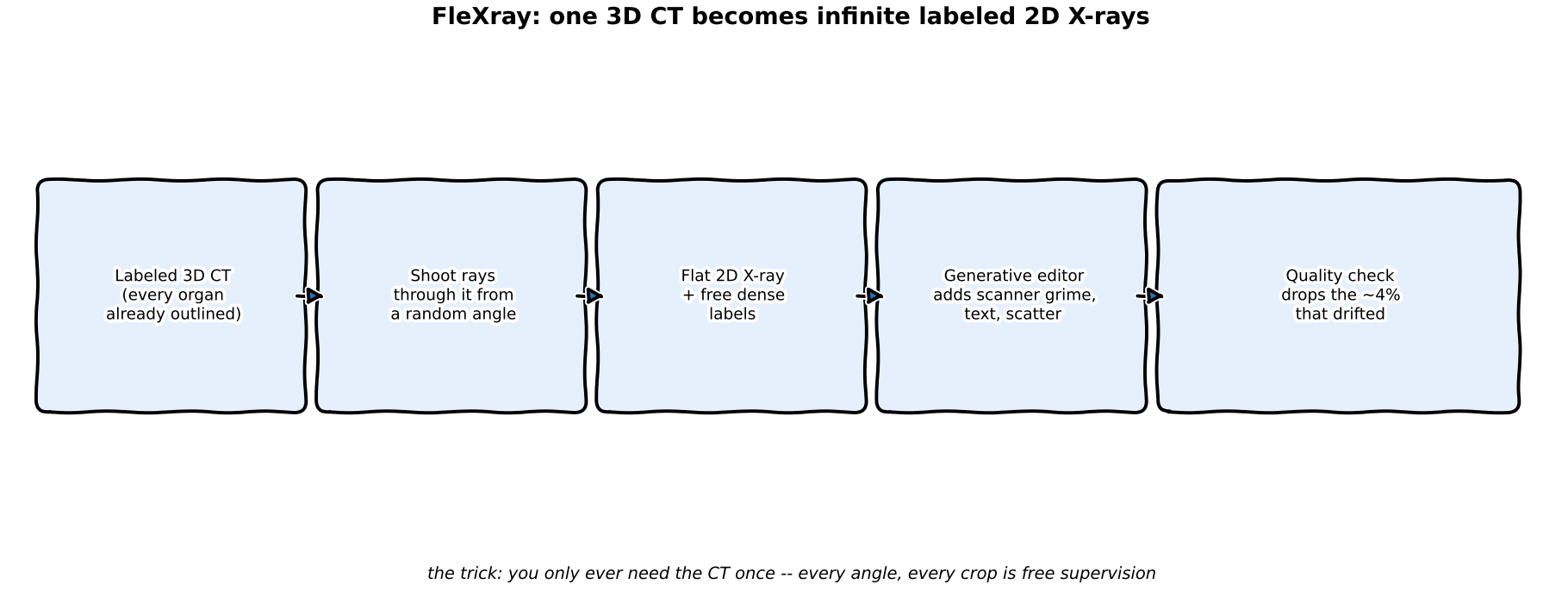
Picture a doctor who has one perfect 3D wax model of a skeleton with every bone already painted a different color. Instead of asking a thousand people to trace bones on a thousand flat photographs (slow, and everyone traces slightly differently), the doctor shines a flashlight through the wax model from a hundred different angles and traces the shadow each time. Because the colors are already painted on the model, every shadow comes with a free, perfect answer key. Then a photo-editing artist roughs up each shadow so it looks like a real, grubby hospital X-ray instead of a clean toy shadow. Do that with a few thousand wax models covering every body type, and you never need a human to trace a real X-ray by hand again.

0.3 Explaining for a data scientist

The engine has three moving parts, and the paper is explicit that none of them alone is sufficient (Appendix E.2.3 ablation, referenced on p.10): physics-based ray projection alone transfers poorly to real radiographs; per-structure attenuation randomization (independently jittering each organ’s simulated density) accounts for most of the domain-gap closing; generative appearance editing adds further benefit specifically where analytic rendering is least faithful (scanner text, contrast agents, implants); and real X-ray data for peripheral anatomy (hands, feet – only 4% of training iterations) closes coverage gaps CT sources simply don’t have (whole-body CT protocols rarely image extremities in frame). Supervision is handled with a dataset-routed loss: because each source dataset only labels a subset of the 60-structure vocabulary, absence in one dataset is not treated as a negative label for structures that dataset never annotated – only structures that are anatomically impossible in a given view (e.g. hand bones in a foot X-ray) are used as explicit negatives. This is what lets six differently-labeled CT sources and four differently-labeled X-ray sources be trained jointly without one dataset’s blank space poisoning another’s positive labels.

0.4 Jargon-buster

Term	Plain meaning
DRR (Digitally Reconstructed Radiograph)	A synthetic X-ray made by ray-summing through a 3D CT volume — a physics simulation of what an X-ray detector would see, not a photo. Think of shining a flashlight through a toy block: the shadow isn’t a photo of the block, it just shows how thickness/density blocks the light.
Attenuation randomization	Independently jittering how much each labeled structure “blocks” the simulated X-ray beam, to cover the real density variation seen across patients (bone disease, contrast agents, implants) without needing real examples of each. Suppose for every flashlight shadow you randomly tint each part of the toy darker or lighter — you learn to handle all the shadow variants you’ll see later.
Dataset-routed loss	A loss function that only penalizes a prediction against the labels its source dataset actually provides, instead of assuming “not labeled” means “absent.” For example, grade a student only on the questions they were given — don’t mark them wrong for answers they never saw.
Label harmonization	Mapping several datasets’ different naming/granularity for the same anatomy (e.g. “spine” vs. “L1 vertebra”) into one shared vocabulary so they can be trained on jointly. Think of merging grocery lists where one says “fruit” and another says “bananas” into one common list that covers both.
Geodesic distance from frontal view	How far off-angle an X-ray was taken from a standard straight-on shot — used here to measure how a model’s accuracy decays as acquisition angle gets more oblique. Think of how much you’ve turned your head away from someone facing you: the bigger the angle, the harder recognition gets.
Test-time augmentation (TTA) + ensembling	Running the same image through the model multiple times with small input variations (and/or through several independently trained models) and averaging the predictions, trading extra inference compute for robustness. Suppose you ask several friends what’s in a blurry photo, also show them slightly different crops, then take the majority answer.
Chamfer loss (in 2D/3D registration)	A distance-based loss that pulls two point sets/contours together — here, aligning a predicted 2D structure boundary to its projected 3D counterpart, used as a smoother, less-local-minima-prone alternative to raw image-similarity optimization. Think of tracing two outlines of the same shape (paper vs. shadow) and shrinking the gap between their borders until they match.

0.5 Architecture — traced from the paper

The pipeline the paper describes, in order. Click a stage (or use the arrow keys once a stage is focused) to walk the engine.

Source pooling

Six CT datasets (2,159 subjects; 1,597 from MOOSE for whole-body coverage) plus five targeted CT sets filling age/anatomy gaps, and four real X-ray sets (764 samples: public hand/foot plus manual forearm/upper-arm from MURA). Extremities are included on purpose — whole-body CT protocols systematically miss them.

0.6 Watch the core idea, run for real

The one mechanism that matters most for a defect-detection use case is the projection step itself: one labeled 3D volume, ray-summed from many angles, produces an unlimited number of labeled 2D X-rays. There’s no public micro-CT-of-castings-with-voids dataset to demonstrate this on real data, so below is the actual mechanism run on a toy synthetic volume – a dense block with two embedded lower-density voids, real numpy/scipy rotation and line-integral projection, 24 real angles:

notebooks/paper-flexray-void/generate_projection_gif.py (core projection loop)

volume = np.zeros((N, N, N), dtype=np.float32)
volume[16:80, 16:80, 16:80] = 1.0          # solid casting block
volume[void_mask] = 0.12                    # embedded low-density void
volume[void2] = 0.12                        # a second, smaller, off-center void

for angle in np.arange(0, 360, 15):
    rotated = rotate(volume, angle=angle, axes=(0, 2), reshape=False, order=1)
    projection = rotated.sum(axis=0)        # parallel-beam line integral
    xray = np.exp(-projection / (vmax * 0.35))   # Beer-Lambert attenuation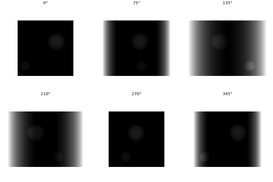

24 real projection angles through a toy volume with two embedded voids – the smaller void (bottom-left) visibly shrinks and nearly disappears at some angles, exactly the acquisition-angle sensitivity the paper measures on real DeepFluoro data (Figure 4b).

This is the entire reusable mechanism, stripped of everything clinical: rotate, sum, threshold. The paper’s real contribution on top of this simple idea is everything that makes the output look like a real acquisition (attenuation randomization, generative appearance editing, QC) rather than a clean toy shadow like the GIF above.

0.7 What FleXray would need to look like for void detection

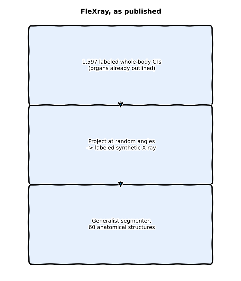
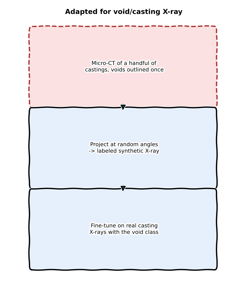
left: FleXray as published  |  right: the same recipe for void/casting X-ray – red dashed box is the ingredient almost nobody in industrial X-ray has

0.8 Does “augmentation” and “editing noise” actually make sense here?

Two questions worth answering with the paper’s own evidence rather than a gut feeling.

Does the broader augmentation pipeline make sense to adopt? Partly, and the paper is precise about which part does the work. FleXray’s augmentation isn’t one thing – it’s geometric/viewpoint randomization (free, from the projection step itself), per-structure attenuation randomization (Ablating attenuation randomization, p.7), and generative appearance editing, each evaluated separately. The paper’s own ablation shows they don’t contribute equally: attenuation randomization moves the equal-dataset mean Dice only modestly (0.863 -> 0.870) in aggregate, but concentrates almost all of its benefit in pathological, density-shifted cases – on DarwinCVD19, lung Dice goes 0.907 -> 0.922 overall, and that gain is entirely in pneumonia cases (0.894 -> 0.914, dense lungs) with the healthy-lung gain essentially flat (0.945 -> 0.946). That’s the useful pattern to copy: density-style augmentation earns its keep specifically on the density-shifted tail of the distribution, not uniformly.

Does adding “editing noise” (generative appearance editing) make sense as augmentation? The paper answers this more precisely than yes/no. When generative editing is treated as pure augmentation (equal proportions of standard vs. enhanced DRRs, p.7-8, “Ablating generative enhancement”), the aggregate equal-dataset Dice is literally unchanged: 0.870 enhanced vs. 0.870 raw (n=1,458). The real gain is concentrated exactly where the analytic renderer already systematically fails to look real – lower ribs obscured by abdominal organs in standard DRRs (Figure 4c): ribs 5-10 all improve with generative enhancement (+3.9 Dice pooled, p<0.001), rising from +2.5 at rib 5 to +7.4 at rib 10. In the paper’s own words, generative editing “contributes useful appearance variation beyond conventional augmentation” – but only where physics-based rendering has a specific, known blind spot, not as a blanket accuracy booster.

That distinction matters more for void detection than it did for FleXray, for a reason the paper doesn’t have to worry about: an organ’s signal is macro-scale; a void’s signal is a small, local attenuation dip. FleXray’s automatic QC is tuned to catch gross anatomical deviation (~4% rejected) – an organ hallucinating a slightly wrong shape is still visually obvious. A generative editor asked to add “scanner grime” to a casting X-ray has an easy, low-cost way to quietly blur or erase a small void while leaving the overall image looking perfectly plausible, and a QC step built to catch gross deviations would not necessarily catch that. So the honest read is: physics-based noise/blur/attenuation modeling (already the approach in Synthetic Data Part 1) should stay the default, and generative “editing noise” is worth the QC overhead only for the specific failure modes physics can’t reach – e.g. a faint void sitting in genuinely noisy cast-surface texture – not as a routine augmentation applied to every synthetic example.

0.9 What I’m taking / skipping for void detection

Personal shortlist — what I’ll actually try, what I won’t, and what sits in the “if time” pile.

Will try:

• Per-structure attenuation randomization is the single most directly reusable idea. A void is a local attenuation deficit – FleXray independently jittering each labeled structure’s simulated density to cover real inter-patient variation maps almost one-to-one onto jittering a synthetic void’s depth/density to cover real porosity variation. This is a concrete refinement to add to Synthetic Data Part 1’s attenuation-depth calibration, not a new idea to adopt wholesale.
• The dataset-routed partial-label loss solves a real, current problem: GDXray alone has castings, welds, and baggage each labeling different defect vocabularies, and combining public industrial X-ray defect datasets (different products, different defect taxonomies) the naive way risks treating one dataset’s unlabeled defect classes as confirmed negatives. Routing supervision per-source, with only anatomically-certain (here: physically-certain) negatives used explicitly, is a clean fix.
• Automatic QC on generative edits is exactly the discipline this blog’s own Qwen-Image-2.1 post needed and didn’t fully have – FleXray’s ~4% rejection-rate number is a concrete target: measure and report the reject rate for any generative-editing step in the void synthesis pipeline, don’t assume every edit is usable.
• Angle-robustness as an evaluation axis, not just accuracy. FleXray’s Dice-vs-geodesic-angle curve (Figure 4b) is a better evaluation habit than a single aggregate metric – a void detector should be measured the same way: accuracy as a function of acquisition angle, not just “AP on the held-out set.”
• Few-shot fine-tuning from a broad synthetic pretrain is the right framing for rare defects. Section “FleXray adapts to unseen segmentation targets” shows the biggest benefit at 1% of real labels, narrowing as real data grows – precisely this series’ own recurring problem (“you can’t collect 500 real examples of a defect type your line sees twice a year,” per the Qwen-Image-2.1 post). The value proposition – broad synthetic pretrain, then fine-tune on a handful of real labeled examples – is directly the shape to aim for, even without CT-scale data.

Will not test:

• The CT-as-ground-truth trick doesn’t have an industrial equivalent at scale. FleXray’s entire engine is downstream of 1,597 already densely labeled whole-body CTs – that abundance is a quirk of medical imaging infrastructure (CT segmentation datasets have been curated for over a decade for radiotherapy planning). There is no equivalent public “micro-CT of castings with voids already outlined” dataset. A handful of industrial CT scans of castings do exist inside companies doing porosity inspection, but nothing at MOOSE’s scale is public. This is the red box in the comparison above, and it’s the load-bearing assumption of the whole paper – without it, the rest of the engine has nothing to project from.
• The 60-structure anatomical taxonomy and harmonization machinery is overkill. Void detection has a handful of defect classes per product family, not 60 overlapping anatomical structures with inter-dataset ontology conflicts. Building FleXray-scale label-harmonization infrastructure for a 3-5 class problem is solving a problem that doesn’t exist yet.
• The clinical downstream applications (Cobb-angle grading, 2D/3D surgical registration) aren’t the shape of the void-detection problem. Void detection is single-shot classification/detection on one acquisition, not iterative registration against a live 3D pose during a procedure. The one place a Chamfer-style registration idea might eventually matter is registering an inspection X-ray against a nominal/golden CAD projection to localize where a casting deviates – worth filing away, not worth building now — maybe later as a follow-up in the Image Registration series.

If time allows:

• The specific backbone/architecture isn’t the point. The paper is explicit that its result is about training distribution design, not architecture (Discussion, p.10: “successful synthetic training depends less on reproducing any single notion of realism than on achieving broad coverage”). Copying FleXray’s network wholesale would import complexity with none of the benefit, since the benefit lives entirely in the data engine. Still, if I get spare cycles, I’ll try their architecture side-by-side with my planned DINO-UNet — as a controlled check that the gains (or lack of them) really come from the data recipe, not the backbone.

0.10 The honest bottom line

FleXray is not a model to adopt for void detection – it’s a proof that attenuation randomization + a partial-label-aware loss + measured generative-editing QC is a data engine design that generalizes well when the source labels are good and broad rather than realistic. The one thing standing between this idea and a real void-detection version of it is the CT-scale labeled 3D source data this domain doesn’t have. The honest next step isn’t “reimplement FleXray for universal defect detection” — it’s take the few transferable pieces above, run them on my own pipeline, and measure whether they move the needle.